Radiosity

FEM (Finite Element Method)

The main idea of FEM (Finite Element Method) is to convert the infinite problem of solving a differential equation into the finite problem of solving a set of simultaneous linear equations.

Let $\displaystyle \operatorname{f}(x)$ be the unknown function of the differential equation $\displaystyle \operatorname{P}(\operatorname{f}(x)) = \operatorname{Q}(\operatorname{f}(x))$.

We try to approximate the $\displaystyle \operatorname{f}(x)$ by the basis functions $\displaystyle \sum_{k=1}^n f_k \operatorname{v_k}(x)$. The idea of the basis functions in FEM is similar to SH (Spherical Harmonics) or Fourier. But since the aim of the FEM is usually to discretize the domain of $\displaystyle \operatorname{f}(x)$, the basis functions in FEM is much simpler than in SH or Fourier. For example, when the domain of $\displaystyle \operatorname{f}(x)$ is [0, 1], let $\displaystyle \operatorname{v_1}(x) = {\begin{cases} 1 &{x \isin [0, \frac{1}{2}]} \\0 &{x \isin [\frac{1}{2}, 1]} \end{cases}}$ and $\displaystyle \operatorname{v_2}(x) = {\begin{cases} 0 &{x \isin [0, \frac{1}{2}]} \\1 &{x \isin [\frac{1}{2}, 1]} \end{cases}}$, evidently $\displaystyle \operatorname{v_1}(x)$ and $\displaystyle \operatorname{v_2}(x)$ are orthogonal.

Let $\displaystyle \operatorname{r}(x) = \operatorname{P}(\sum_{k=1}^n f_k \operatorname{v_k}(x)) - \operatorname{Q}(\sum_{k=1}^n f_k \operatorname{v_k}(x))$ be the residual. The projection of the residual onto each basis function should be zero. This means that, for each i = 1 ... n, we have the equation $\displaystyle \int \operatorname{r}(x) \operatorname{v_i}(x) = \int \left\lparen \operatorname{P}(\sum_{j=1}^n f_j \operatorname{v_j}(x)) - \operatorname{Q}(\sum_{j=1}^n f_j \operatorname{v_j}(x)) \right\rparen \operatorname{v_i}(x) = 0$ of which the result is essentially a linear equation about the n coefficients $\displaystyle f_j$ . And these n linear equations are composed as the simultaneous linear equations about the n coefficients $\displaystyle f_j$ .

Note that the basis function $\displaystyle \operatorname{v_i}(x)$ is also called the weight function or test function, the $\displaystyle \operatorname{R}(x) = \operatorname{r}(x) \operatorname{v_i}(x)$ is also called the weighted residual, and the linear equation $\displaystyle \int \operatorname{r}(x) \operatorname{v_i}(x) = 0$ is also called the variational form or the weak form in FreeFEM.

Rendering Equation

The Rendering Equation is also called the LTE (Light Transport Equation) by "14.4 The Light Transport Equation" of PBR Book V3. And we have the Rendering Equation $\displaystyle \operatorname{L_o}(\overrightarrow{p}, \overrightarrow{\omega_o}) = \operatorname{L_e}(\overrightarrow{p}, \overrightarrow{\omega_o}) + \int_\Omega \operatorname{f}(\overrightarrow{p}, \overrightarrow{\omega_i}, \overrightarrow{\omega_o}) \operatorname{L_i}(\overrightarrow{p}, \overrightarrow{\omega_i}) (\cos \theta_i)^+ \, d \overrightarrow{\omega_i}$ .

According to the Rendering Equation, by OSL (Open Shading Language), the surface and the light are actually the same thing, since the light is merely the surface which is emissive.

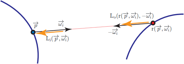
By "Figure 11.1" of Real-Time Rendering Fourth Edition and "Figure 14.14" of PBR Book V3, by assuming no participating media, we have the relationship $\displaystyle \operatorname{L_i}(\overrightarrow{p}, \overrightarrow{\omega_i}) = \operatorname{L_o}(\operatorname{r}(\overrightarrow{p}, \overrightarrow{\omega_i}), -\overrightarrow{\omega_i})$ where $\displaystyle \operatorname{r}(\overrightarrow{p}, \overrightarrow{\omega})$ is the ray-casting function. This means that the incident radiance $\displaystyle \operatorname{L_i}(\overrightarrow{p}, \overrightarrow{\omega_i})$ at one point p is exactly the exitant radiance $\displaystyle \operatorname{L_o}(\operatorname{r}(\overrightarrow{p}, \overrightarrow{\omega_i}), -\overrightarrow{\omega_i})$ at another point $\displaystyle \operatorname{r}(\overrightarrow{p}, \overrightarrow{\omega_i})$.

Hence, both the incident radiance $\displaystyle \operatorname{L_i}(\overrightarrow{p}, \overrightarrow{\omega})$ and the exitant radiance $\displaystyle \operatorname{L_o}(\overrightarrow{p}, \overrightarrow{\omega})$ can be represented by the same function $\displaystyle \operatorname{L}(\overrightarrow{p}, \overrightarrow{\omega})$. And thus, we have $\displaystyle \operatorname{L}(\overrightarrow{p}, \overrightarrow{\omega_o}) = \operatorname{L_e}(\overrightarrow{p}, \overrightarrow{\omega_o}) + \int_\Omega \operatorname{f}(\overrightarrow{p}, \overrightarrow{\omega_i}, \overrightarrow{\omega_o}) \operatorname{L}(\operatorname{r}(\overrightarrow{p}, \overrightarrow{\omega_i}), -\overrightarrow{\omega_i}) (\cos \theta_i)^+ \, d \overrightarrow{\omega_i}$ which is a differential equation of which the unknown function is the $\displaystyle \operatorname{L}(\overrightarrow{p}, \overrightarrow{\omega})$.

Thus, the problem of rendering is essentially a problem of solving the differential equation. There are two independent approaches: ray tracing (which depends on the Fredholm theory) and radiosity (which depends on the FEM).

Ray Tracing

By "Light transport and the rendering equation" of CS 348B - Computer Graphics: Image Synthesis Techniques and "Global Illumination and Rendering Equation" of CS 294-13 Advanced Computer Graphics, this differential equation is actually the Fredholm Integral Equation of which the solution is the Liouville–Veumann Series. And thus, the solution of this differential equation can be written as the recursive form $\text{L} = \text{E} + \text{K}\text{E} + {\text{K}}^2\text{E} + {\text{K}}^3\text{E} + \ldots$ .

Radiosity

Note that the term radiosity B has been deprecated and should be called radiant exitance M or outgoing irradiance E instead. But to be consistent with most literature about radiosity, we still use radiosity B here.

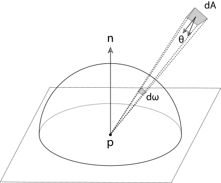
By "Equation (5.6)" of PBR Book V3, we have the relationship $\displaystyle d\omega = \frac{\cos\theta}{r^2} dA$.

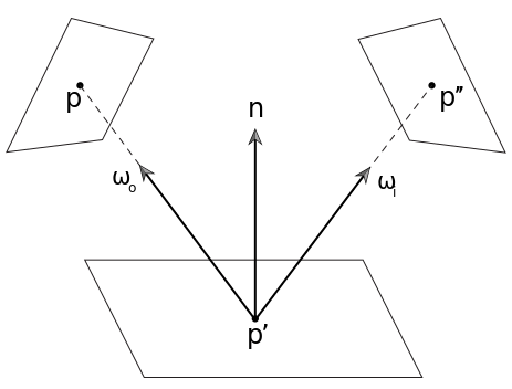
By "Equation (14.14)" of PBR Book V3, let $\operatorname{V}$ be the visibility function and we have the surface form of the rendering equation $\displaystyle \operatorname{L}(\overrightarrow{p'} \rightarrow \overrightarrow{p}) = \operatorname{L_e}(\overrightarrow{p'} \rightarrow \overrightarrow{p}) + \int_A \operatorname{f}(\overrightarrow{p''} \rightarrow \overrightarrow{p'} \rightarrow \overrightarrow{p}) \operatorname{V}(\overrightarrow{p''} \leftrightarrow \overrightarrow{p'}) \operatorname{L}(\overrightarrow{p''} \rightarrow \overrightarrow{p'}) (\cos \theta')^+ \frac{(\cos \theta'')^+}{{\| \overrightarrow{p''} - \overrightarrow{p'} \|}^2} \, d \operatorname{A}(\overrightarrow{p''}) = \operatorname{L_e}(\overrightarrow{p'} \rightarrow \overrightarrow{p}) + \int_A \operatorname{f}(\overrightarrow{p''} \rightarrow \overrightarrow{p'} \rightarrow \overrightarrow{p}) \operatorname{L}(\overrightarrow{p''} \rightarrow \overrightarrow{p'}) \operatorname{G}(\overrightarrow{p''} \rightarrow \overrightarrow{p'}) \, d \operatorname{A}(\overrightarrow{p''})$ where integral interval $\displaystyle A$ is the area of all the surfaces in the scene and $\displaystyle \operatorname{G}(\overrightarrow{p''} \rightarrow \overrightarrow{p'}) = \operatorname{V}(\overrightarrow{p''} \leftrightarrow \overrightarrow{p'}) \frac{(\cos \theta')^+ (\cos \theta'')^+}{{\| \overrightarrow{p''} - \overrightarrow{p'} \|}^2}$.

We assume that the Lambert BRDF $\displaystyle \operatorname{f}(\overrightarrow{p''} \rightarrow \overrightarrow{p'} \rightarrow \overrightarrow{p}) = \frac{1}{\pi} \operatorname{\rho_{hd}}(\overrightarrow{p'})$ is used. This means that the outgoing radiance is the same in all directions and we have the relationship $\displaystyle \operatorname{L}(\overrightarrow{p'} \rightarrow \overrightarrow{p}) = \frac{\operatorname{B}(\overrightarrow{p'})}{\pi}$ where the $\displaystyle \operatorname{B}(\overrightarrow{p'})$ does NOT depend on the direction $\displaystyle \overrightarrow{p'} \rightarrow \overrightarrow{p}$ . Hence, by "Equation (2.54)" of [Cohen 1993], the rendering equation can be written as the radiosity equation $\displaystyle \frac{\operatorname{B}(\overrightarrow{p'})}{\pi} = \frac{\operatorname{B_e}(\overrightarrow{p'})}{\pi} + \int_A \frac{1}{\pi} \operatorname{\rho_{hd}}(\overrightarrow{p'}) \frac{\operatorname{B}(\overrightarrow{p''})}{\pi} \operatorname{G}(\overrightarrow{p''} \rightarrow \overrightarrow{p'}) \, d \operatorname{A}(\overrightarrow{p''})$ ⇒ $\displaystyle \operatorname{B}(\overrightarrow{p'}) = \operatorname{B_e}(\overrightarrow{p'}) + \frac{1}{\pi} \operatorname{\rho_{hd}}(\overrightarrow{p'}) \int_A \operatorname{B}(\overrightarrow{p''}) \operatorname{G}(\overrightarrow{p''} \rightarrow \overrightarrow{p'}) \, d \operatorname{A}(\overrightarrow{p''})$ ⇒ $\displaystyle \operatorname{B}(\overrightarrow{p}) = \operatorname{B_e}(\overrightarrow{p}) + \frac{1}{\pi} \operatorname{\rho_{hd}}(\overrightarrow{p}) \int_A \operatorname{B}(\overrightarrow{p'}) \operatorname{G}(\overrightarrow{p'} \rightarrow \overrightarrow{p}) \, d \operatorname{A}(\overrightarrow{p'})$.

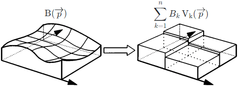
By "Equation (3.2)" of [Cohen 1993], by FEM, the surface is discretized into n patches, and the solution of the radiosity equation $\displaystyle \operatorname{B}(\overrightarrow{p})$ is approximated by n basis functions $\displaystyle \sum_{k=1}^n B_k \operatorname{V_k}(\overrightarrow{p})$. And by "Equation (3.3)" of [Cohen 1993], the basis function can be as simple as the constant basis function, which is the P0 Element in FreeFEM, $\displaystyle \operatorname{V_k}(\overrightarrow{p}) = {\begin{cases} 1 &{\overrightarrow{p} \isin A_k} \\0 &{\overrightarrow{p} \notin A_k} \end{cases}}$ where $\displaystyle A_k$ is the area of the k-th patch surface.

By "Equation (3.4)" of [Cohen 1993], we have the residual $\displaystyle \operatorname{r}(\overrightarrow{p}) = \sum_{j=1}^n B_j \operatorname{V_j}(\overrightarrow{p}) - \left \lparen \operatorname{B_e}(\overrightarrow{p}) + \frac{1}{\pi} \operatorname{\rho_{hd}}(\overrightarrow{p}) \int_A \left \lparen \sum_{j=1}^n B_j \operatorname{V_j}(\overrightarrow{p}) \right \rparen \operatorname{G}(\overrightarrow{p'} \rightarrow \overrightarrow{p}) \, d \operatorname{A}(\overrightarrow{p'}) \right \rparen = \sum_{j=1}^n B_j \operatorname{V_j}(\overrightarrow{p}) - \operatorname{B_e}(\overrightarrow{p}) - \frac{1}{\pi} \operatorname{\rho_{hd}}(\overrightarrow{p}) \int_A \left \lparen \sum_{j=1}^n B_j \operatorname{V_j}(\overrightarrow{p}) \right \rparen \operatorname{G}(\overrightarrow{p'} \rightarrow \overrightarrow{p}) \, d \operatorname{A}(\overrightarrow{p'})$.

By "Equation (3.19)" of [Cohen 1993], the projection of the residual onto each basis function should be zero. This means that, for each i = 1 ... n, we have the linear equation about the n coefficients $\displaystyle B_j$ $\displaystyle 0 = \int_A \operatorname{r}(\overrightarrow{p}) \operatorname{V_i}(\overrightarrow{p}) \, d \operatorname{A}(\overrightarrow{p}) = \int_A \left \lparen \sum_{j=1}^n B_j \operatorname{V_j}(\overrightarrow{p}) - \operatorname{B_e}(\overrightarrow{p}) - \frac{1}{\pi} \operatorname{\rho_{hd}}(\overrightarrow{p}) \int_A \left \lparen \sum_{j=1}^n B_j \operatorname{V_j}(\overrightarrow{p}) \right \rparen \operatorname{G}(\overrightarrow{p'} \rightarrow \overrightarrow{p}) \, d \operatorname{A}(\overrightarrow{p'}) \right \rparen \operatorname{V_i}(\overrightarrow{p}) \, d \operatorname{A}(\overrightarrow{p}) = B_i A_i - B_i^e A_i - A_i \rho_i^{hd} \sum_{j=1}^n F_{ij} B_j$ where $\displaystyle A_i$ is the area of the i-th patch surface, $\displaystyle \operatorname{B_e}(\overrightarrow{p})$ is the assumed to be the constant $\displaystyle B_i^e$ over the i-th patch surface, $\displaystyle \operatorname{\rho_{hd}}(\overrightarrow{p})$ is the assumed to be the constant $\displaystyle \rho_i^{hd}$ over the i-th patch surface and $\displaystyle F_{ij} = \frac{1}{A_i} \frac{1}{\pi} \int_{A_i} \int_{A_j} \operatorname{G}(\overrightarrow{p'} \rightarrow \overrightarrow{p}) \, d \operatorname{A}(\overrightarrow{p'}) \, d \operatorname{A}(\overrightarrow{p})$ is the form factor. This means that $\displaystyle B_i = B_i^e + \rho_i^{hd} \sum_{j=1}^n F_{ij} B_j$ which is exactly the "Equation (11.4)" of Real-Time Rendering Fourth Edition.

Proof

By Linearity Property, we have $\displaystyle \int_A \left \lparen \sum_{j=1}^n B_j \operatorname{V_j}(\overrightarrow{p}) - \operatorname{B_e}(\overrightarrow{p}) - \frac{1}{\pi} \operatorname{\rho_{hd}}(\overrightarrow{p}) \int_A \left \lparen \sum_{j=1}^n B_j \operatorname{V_j}(\overrightarrow{p}) \right \rparen \operatorname{G}(\overrightarrow{p'} \rightarrow \overrightarrow{p}) \, d \operatorname{A}(\overrightarrow{p'}) \right \rparen \operatorname{V_i}(\overrightarrow{p}) \, d \operatorname{A}(\overrightarrow{p}) = \int_A \left \lparen \sum_{j=1}^n B_j \operatorname{V_j}(\overrightarrow{p}) \right \rparen \operatorname{V_i}(\overrightarrow{p}) \, d \operatorname{A}(\overrightarrow{p}) - \int_A \operatorname{B_e}(\overrightarrow{p}) \operatorname{V_i}(\overrightarrow{p}) \, d \operatorname{A}(\overrightarrow{p}) - \int_A \left \lparen \frac{1}{\pi} \operatorname{\rho_{hd}}(\overrightarrow{p}) \int_A \left \lparen \sum_{j=1}^n B_j \operatorname{V_j}(\overrightarrow{p}) \right \rparen \operatorname{G}(\overrightarrow{p'} \rightarrow \overrightarrow{p}) \, d \operatorname{A}(\overrightarrow{p'}) \right \rparen \operatorname{V_i}(\overrightarrow{p}) \, d \operatorname{A}(\overrightarrow{p})$

First, we would like to prove that $\displaystyle \int_A \left \lparen \sum_{j=1}^n B_j \operatorname{V_j}(\overrightarrow{p}) \right \rparen \operatorname{V_i}(\overrightarrow{p}) \, d \operatorname{A}(\overrightarrow{p}) = B_i A_i$ .

By Linearity Property, we have $\displaystyle \int_A \left \lparen \sum_{j=1}^n B_j \operatorname{V_j}(\overrightarrow{p}) \right \rparen \operatorname{V_i}(\overrightarrow{p}) \, d \operatorname{A}(\overrightarrow{p}) = \sum_{j=1}^n \int_A B_j \operatorname{V_j}(\overrightarrow{p}) \operatorname{V_i}(\overrightarrow{p}) \, d \operatorname{A}(\overrightarrow{p})$.
Since $\displaystyle \operatorname{V_j}(\overrightarrow{p}) = {\begin{cases} 1 &{\overrightarrow{p} \isin A_j} \\0 &{\overrightarrow{p} \notin A_j} \end{cases}}$ , we have $\displaystyle \sum_{j=1}^n \int_A B_j \operatorname{V_j}(\overrightarrow{p}) \operatorname{V_i}(\overrightarrow{p}) \, d \operatorname{A}(\overrightarrow{p}) = \int_A B_i \operatorname{V_i}(\overrightarrow{p}) \operatorname{V_i}(\overrightarrow{p}) \, d \operatorname{A}(\overrightarrow{p}) = \int_{A_i} B_i \, d \operatorname{A}(\overrightarrow{p}) = B_i A_i$

Second, we would like to prove that $\displaystyle \int_A \operatorname{B_e}(\overrightarrow{p}) \operatorname{V_i}(\overrightarrow{p}) \, d \operatorname{A}(\overrightarrow{p}) = B_i^e A_i$ .

Since $\displaystyle \operatorname{V_j}(\overrightarrow{p}) = {\begin{cases} 1 &{\overrightarrow{p} \isin A_j} \\0 &{\overrightarrow{p} \notin A_j} \end{cases}}$ , we have $\displaystyle \int_A \operatorname{B_e}(\overrightarrow{p}) \operatorname{V_i}(\overrightarrow{p}) \, d \operatorname{A}(\overrightarrow{p}) = \int_{A_i} \operatorname{B_e}(\overrightarrow{p}) \, d \operatorname{A}(\overrightarrow{p})$.
Since $\displaystyle \operatorname{B_e}(\overrightarrow{p})$ is the assumed to be the constant $\displaystyle B_i^e$ over the ith patch surface, we have $\displaystyle \int_{A_i} \operatorname{B_e}(\overrightarrow{p}) \, d \operatorname{A}(\overrightarrow{p}) = B_i^e A_i$ .

Third, we would like to prove that $\displaystyle \int_A \left \lparen \frac{1}{\pi} \operatorname{\rho_{hd}}(\overrightarrow{p}) \int_A \left \lparen \sum_{j=1}^n B_j \operatorname{V_j}(\overrightarrow{p}) \right \rparen \operatorname{G}(\overrightarrow{p'} \rightarrow \overrightarrow{p}) \, d \operatorname{A}(\overrightarrow{p'}) \right \rparen \operatorname{V_i}(\overrightarrow{p}) \, d \operatorname{A}(\overrightarrow{p}) = A_i \rho_i^{hd} \sum_{j=1}^n F_{ij} B_j$ .

By Linearity Property, we have $\displaystyle \int_A \left \lparen \frac{1}{\pi} \operatorname{\rho_{hd}}(\overrightarrow{p}) \int_A \left \lparen \sum_{j=1}^n B_j \operatorname{V_j}(\overrightarrow{p}) \right \rparen \operatorname{G}(\overrightarrow{p'} \rightarrow \overrightarrow{p}) \, d \operatorname{A}(\overrightarrow{p'}) \right \rparen \operatorname{V_i}(\overrightarrow{p}) \, d \operatorname{A}(\overrightarrow{p}) = \sum_{j=1}^n \int_A \left \lparen \frac{1}{\pi} \operatorname{\rho_{hd}}(\overrightarrow{p}) \int_A B_j \operatorname{V_j}(\overrightarrow{p}) \operatorname{G}(\overrightarrow{p'} \rightarrow \overrightarrow{p}) \, d \operatorname{A}(\overrightarrow{p'}) \right \rparen \operatorname{V_i}(\overrightarrow{p}) \, d \operatorname{A}(\overrightarrow{p})$.
Since $\displaystyle \operatorname{V_i}(\overrightarrow{p}) = {\begin{cases} 1 &{\overrightarrow{p} \isin A_i} \\0 &{\overrightarrow{p} \notin A_i} \end{cases}}$ and $\displaystyle \operatorname{V_j}(\overrightarrow{p}) = {\begin{cases} 1 &{\overrightarrow{p} \isin A_j} \\0 &{\overrightarrow{p} \notin A_j} \end{cases}}$ , we have $\displaystyle \sum_{j=1}^n \int_A \left \lparen \frac{1}{\pi} \operatorname{\rho_{hd}}(\overrightarrow{p}) \int_A B_j \operatorname{V_j}(\overrightarrow{p}) \operatorname{G}(\overrightarrow{p'} \rightarrow \overrightarrow{p}) \, d \operatorname{A}(\overrightarrow{p'}) \right \rparen \operatorname{V_i}(\overrightarrow{p}) \, d \operatorname{A}(\overrightarrow{p}) = \sum_{j=1}^n \int_{A_i} \left \lparen \frac{1}{\pi} \operatorname{\rho_{hd}}(\overrightarrow{p}) \int_{A_j} B_j \operatorname{G}(\overrightarrow{p'} \rightarrow \overrightarrow{p}) \, d \operatorname{A}(\overrightarrow{p'}) \right \rparen \, d \operatorname{A}(\overrightarrow{p})$.
Since $\displaystyle \operatorname{\rho_{hd}}(\overrightarrow{p})$ is the assumed to be the constant $\displaystyle \rho_i^{hd}$ over the ith patch surface, we have $\displaystyle \sum_{j=1}^n \int_{A_i} \left \lparen \frac{1}{\pi} \operatorname{\rho_{hd}}(\overrightarrow{p}) \int_{A_j} B_j \operatorname{G}(\overrightarrow{p'} \rightarrow \overrightarrow{p}) \, d \operatorname{A}(\overrightarrow{p'}) \right \rparen \, d \operatorname{A}(\overrightarrow{p}) = \rho_i^{hd} \sum_{j=1}^n \frac{1}{\pi} B_j \int_{A_i} \left \lparen \int_{A_j} \operatorname{G}(\overrightarrow{p'} \rightarrow \overrightarrow{p}) \, d \operatorname{A}(\overrightarrow{p'}) \right \rparen \, d \operatorname{A}(\overrightarrow{p}) = A_i \rho_i^{hd} \sum_{j=1}^n \left \lparen \frac{1}{A_i} \frac{1}{\pi} \int_{A_i} \int_{A_j} \operatorname{G}(\overrightarrow{p'} \rightarrow \overrightarrow{p}) \, d \operatorname{A}(\overrightarrow{p'}) \, d \operatorname{A}(\overrightarrow{p}) \right \rparen B_j = A_i \rho_i^{hd} \sum_{j=1}^n F_{ij} B_j$

References

[Cohen 1993] Michael Cohen, John Wallace. "Radiosity and Realistic Image Synthesis." Academic Press Professional 1993.
[Hecht 2012] Frederic Hecht. "New development in FreeFem++." Journal of Numerical Mathematics 2012.