DLB (Dual Quaternion Linear Blending)

1. Linear Blending

The main idea of the linear blending method is to calculate the linear combination of the joint (bone) matrices. By [Kavan 2007] and [Kavan 2008], the rigid transform is the composition of rotation transform and translation transform. Evidently, the linear blending method is NOT correct, since the linear combination of the rigid transformation matrices is NOT necessarily a rigid transformation matrix. However, the linear blending method is still one of the most popular vertex blending methods. By [Kavan 2007] and [Kavan 2008], perhaps this is only because there is no simple alternative.

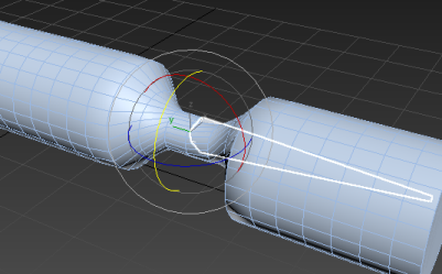
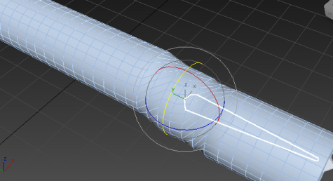
By the documents of Autodesk 3ds Max, we have the "candy-wrapper" artifact of the linear blending.

2. Dual Quaternion Mathematics

2-1. Quaternion

By "Equation (5.3)" of Quaternions for Computer Graphics, a quaternion can be written as $\displaystyle \boldsymbol{q} = w + xi + yj + zk = \begin{bmatrix}s, & \overrightarrow{v}\end{bmatrix}$ where $\displaystyle s = w$ is a real number and $\displaystyle \overrightarrow{v} = \begin{bmatrix}x, & y, & z\end{bmatrix}$ is a vector in 3D space.

2-1-1. Multiplication

By "Equation (5.9)" of Quaternions for Computer Graphics, we have the multiplication of quaternions $\displaystyle \boldsymbol{q_0}\boldsymbol{q_1} = \begin{bmatrix}s_0, & \overrightarrow{v_0}\end{bmatrix} \begin{bmatrix}s_1, & \overrightarrow{v_1}\end{bmatrix} = \begin{bmatrix}s_0 s_1 - \overrightarrow{v_0} \cdot \overrightarrow{v_1}, & s_0 \overrightarrow{v_1} + s_1 \overrightarrow{v_0} + \overrightarrow{v_0} \times \overrightarrow{v_1}\end{bmatrix}$.

2-1-2. Inner Product

By Inner Product Space of Wikipedia, we have the inner product of the quaternions $\langle \boldsymbol{q_0}, \boldsymbol{q_1} \rangle = \langle \begin{bmatrix}s_0, & \overrightarrow{v_0}\end{bmatrix}, \begin{bmatrix}s_1, & \overrightarrow{v_1}\end{bmatrix} \rangle = s_0 s_1 + \overrightarrow{v_0} \cdot \overrightarrow{v_1} = w_0 w_1 + x_0 x_1 + y_0 y_1 + z_0 z_1$ .

2-1-3. Conjugate

By "5.12 The Conjugate" of Quaternions for Computer Graphics, we have the conjugate of a quaternion ${\boldsymbol{q}}^* = {\begin{bmatrix}s, & \overrightarrow{v}\end{bmatrix}}^* = \begin{bmatrix}s, & -\overrightarrow{v}\end{bmatrix}$.

2-1-3-1. Distributive Property

By the multiplication of quaternions, we have that $\displaystyle {(\boldsymbol{q_0} \boldsymbol{q_1})}^* = {\boldsymbol{q_1}}^* {\boldsymbol{q_0}}^*$ . The lengthy calculation is provided by "Equation (5.10)" and "Equation (5.11)" of Quaternions for Computer Graphics.

2-1-4. Norm

By "5.12 The Conjugate" of Quaternions for Computer Graphics, we have the norm of a quaternion $\displaystyle {\| \boldsymbol{q} \|}^2 = \boldsymbol{q} {\boldsymbol{q}}^* = \begin{bmatrix}s, & \overrightarrow{v}\end{bmatrix} \begin{bmatrix}s, & -\overrightarrow{v}\end{bmatrix} = \begin{bmatrix}s^2 - \overrightarrow{v} \cdot (-\overrightarrow{v}), & s (-\overrightarrow{v}) + s \overrightarrow{v} + \overrightarrow{v} \times (-\overrightarrow{v})\end{bmatrix} = \begin{bmatrix}s^2 + {|\overrightarrow{v}|}^2, & \overrightarrow{0}\end{bmatrix} = s^2 + {\| \overrightarrow{v} \|}^2 = w^2 + x^2 + y^2 + z^2 = \langle \boldsymbol{q}, \boldsymbol{q} \rangle \Rightarrow \| \boldsymbol{q} \| = \sqrt{\langle \boldsymbol{q}, \boldsymbol{q} \rangle}$ .

2-1-5. Unit Quaternion

By "5.14 Normalised Quaternion" of Quaternions for Computer Graphics, a unit quaternion is a quaternion of which the norm is one.

2-1-6. Inverse

By "5.16 Inverse Quaternion" of Quaternions for Computer Graphics, we have the inverse of the quaternion $\displaystyle \boldsymbol{q} {\boldsymbol{q}}^{-1} = 1 = \begin{bmatrix}1, & \overrightarrow{0}\end{bmatrix} \Rightarrow {\boldsymbol{q}}^* \boldsymbol{q} {\boldsymbol{q}}^{-1} = {\boldsymbol{q}}^* \Rightarrow ({\boldsymbol{q}}^* \boldsymbol{q}) {\boldsymbol{q}}^{-1} = {\boldsymbol{q}}^* \Rightarrow {\| \boldsymbol{q} \|}^2 {\boldsymbol{q}}^{-1} = {\boldsymbol{q}}^* \Rightarrow {\boldsymbol{q}}^{-1} = \frac{{\boldsymbol{q}}^*}{{\| \boldsymbol{q} \|}^2}$.

2-1-7. Bijection between Rotation Transforms and Unit Quaternions

Each rotation transform can be represented by a unit quaternion, and conversely, each unit quaternion can represent a rotation transform.

2-1-7-1. Mapping the Rotation Transform to the Unit Quaternion

Let $\displaystyle \boldsymbol{q} = \begin{bmatrix}\cos \frac{\theta}{2}, & \sin \frac{\theta}{2} \overrightarrow{n}\end{bmatrix}$ where $\displaystyle \overrightarrow{n}$ is a unit vector in 3D space.

First, we would like to prove that $\displaystyle \boldsymbol{q}$ is a unit quaternion.

The norm of of $\displaystyle \boldsymbol{q}$ is calculated as $\displaystyle {\| \boldsymbol{q} \|}^2 = \cos^2 \frac{\theta}{2} + \sin^2 \frac{\theta}{2} {| \overrightarrow{n} |}^2 = \cos^2 \frac{\theta}{2} + \sin^2 \frac{\theta}{2} = 1$. This means that the norm of $\displaystyle \boldsymbol{q}$ is one. And thus, $\displaystyle \boldsymbol{q}$ is a unit quaternion.

Second, we would like to prove that $\displaystyle \boldsymbol{q}$ represents the rotation transform about the axis $\displaystyle \overrightarrow{n}$ by the angle $\displaystyle \theta$.

Let $\displaystyle \boldsymbol{p} = \begin{bmatrix}0, & \overrightarrow{p}\end{bmatrix}$ where $\displaystyle \overrightarrow{p}$ is the position in 3D space.

Let $\displaystyle \boldsymbol{p'} = \boldsymbol{q} \boldsymbol{p} {\boldsymbol{q}}^{-1} = \begin{bmatrix}s', \overrightarrow{p'}\end{bmatrix}$ where $\displaystyle \overrightarrow{p'}$ is the new position of the position $\displaystyle \overrightarrow{p}$ after the transfrom. Actually, we will later prove that we always have $\displaystyle s' = 0$. Thus, this variable can be ignored.

The inverse of of $\displaystyle \boldsymbol{q}$ is calculated as $\displaystyle {\boldsymbol{q}}^{-1} = \frac{\begin{bmatrix}\cos \frac{\theta}{2}, & - \sin \frac{\theta}{2} \overrightarrow{n}\end{bmatrix}}{{\| \boldsymbol{q} \|}^2} = \begin{bmatrix}\cos \frac{\theta}{2}, & - \sin \frac{\theta}{2} \overrightarrow{n}\end{bmatrix}$.

By the multiplication of quaternions, we have that $\displaystyle \boldsymbol{p'} = \boldsymbol{q} \boldsymbol{p} {\boldsymbol{q}}^{-1} = \begin{bmatrix}\cos \frac{\theta}{2}, & \sin \frac{\theta}{2} \overrightarrow{n}\end{bmatrix} \begin{bmatrix}0, & \overrightarrow{p}\end{bmatrix} \begin{bmatrix}\cos \frac{\theta}{2}, & - \sin \frac{\theta}{2} \overrightarrow{n}\end{bmatrix} = \begin{bmatrix}0, & (1 - \cos \theta) (\overrightarrow{n} \cdot \overrightarrow{p}) \overrightarrow{p} + \cos \theta \overrightarrow{p} + \sin \theta \overrightarrow{n} \times \overrightarrow{p}\end{bmatrix}$. The lengthy calculation is provided by "Equation (7.13)" of Quaternions for Computer Graphics. This means that $\displaystyle s' = 0$ and $\displaystyle \overrightarrow{p'} = (1 - \cos \theta) (\overrightarrow{n} \cdot \overrightarrow{p}) \overrightarrow{p} + \cos \theta \overrightarrow{p} + \sin \theta \overrightarrow{n} \times \overrightarrow{p}$ .

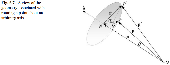
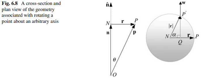
By "Fig. 6.7" and "Fig. 6.8" of Quaternions for Computer Graphics, we have $\displaystyle \overrightarrow{p'}$ is exactly the new position of the position $\displaystyle \overrightarrow{p}$ after the rotation transform about the axis $\displaystyle \overrightarrow{n}$ by the angle $\displaystyle \theta$.

Proof

TODO

2-1-7-2. Mapping the Unit Quaternion to the Rotation Transform

Let $\displaystyle \boldsymbol{q} = \begin{bmatrix}s, & \overrightarrow{v}\end{bmatrix}$ be the unit quaternion, namely, $\displaystyle s^2 + {\| \overrightarrow{v} \|}^2 = 1$.

We would like to prove that there exists the $\displaystyle \theta$ and the $\overrightarrow{n}$ such that $\displaystyle \boldsymbol{q} = \begin{bmatrix}\cos \frac{\theta}{2}, & \sin \frac{\theta}{2} \overrightarrow{n}\end{bmatrix}$ and $\displaystyle \overrightarrow{n}$ is a unit vector in 3D space.

Since $\displaystyle s^2 + {\| \overrightarrow{v} \|}^2 = 1$, we can find the $\displaystyle \theta$ such that $\displaystyle \cos \frac{\theta}{2} = s$ and $\displaystyle \sin \frac{\theta}{2} = \| \overrightarrow{v} \|$. And let $\displaystyle \overrightarrow{n} = \frac{\overrightarrow{v}}{\| \overrightarrow{v} \|}$. Thus, we have that $\displaystyle \boldsymbol{q} = \begin{bmatrix}\cos \frac{\theta}{2}, & \sin \frac{\theta}{2} \overrightarrow{n}\end{bmatrix} = \begin{bmatrix}s, & \overrightarrow{v}\end{bmatrix}$.

This means that the rotation transform about the axis $\displaystyle \overrightarrow{n}$ by the angle $\displaystyle \theta$ is the rotation transform represented by the unit quaternion $\displaystyle \boldsymbol{q}$.

2-2. Dual Numbder

By "A.1 Dual Numbers" of [Kavan 2008], a dual number can be written as $\displaystyle \hat{a} = a_0 + a_\epsilon \epsilon$, where $\displaystyle a_0$ and $\displaystyle a_\epsilon$ are real numbers, and $\displaystyle \epsilon$ is a basis element such that $\displaystyle 1 \epsilon = \epsilon 1 = \epsilon$ and $\epsilon \epsilon = 0$.

2-2-1. Multiplication

By "Equation (17)" of [Kavan 2008], we have the multiplication of dual numbers $\displaystyle \hat{a} \hat{b} = (a_0 + a_\epsilon \epsilon)(b_0 + b_\epsilon \epsilon) = a_0 b_0 + (a_0 b_\epsilon + b_0 a_\epsilon) \epsilon$.

2-2-2. Conjugate

By "A.1 Dual Numbers" of [Kavan 2008], we have the conjugate of a dual number $\displaystyle \overline{\hat{a}} = \overline{a_0 + a_\epsilon \epsilon} = a_0 - a_\epsilon \epsilon$.

2-2-2-1. Distributive Property

By "Lemma 6" of [Kavan 2008], we have that $\displaystyle \overline{\hat{a} \hat{b}} = \overline{\hat{a}} \overline{\hat{b}}$ .

Proof

By the multiplication of dual numbers, we have that $\displaystyle \overline{\hat{a} \hat{b}} = \overline{(a_0 + a_\epsilon \epsilon)(b_0 + b_\epsilon \epsilon)} = \overline{a_0 b_0 + (a_0 b_\epsilon + b_0 a_\epsilon) \epsilon} = a_0 b_0 - (a_0 b_\epsilon + b_0 a_\epsilon) \epsilon = (a_0 - a_\epsilon \epsilon)(b_0 - b_\epsilon \epsilon) = \overline{\hat{a}} \overline{\hat{b}}$ .

2-2-3. Square Root

By "Equation (19)" of [Kavan 2008], for any dual number $\displaystyle \hat{a} = a_0 + a_\epsilon \epsilon$ such that $\displaystyle a_0 \gt 0$, we have the square root of the dual number $\displaystyle \sqrt{\hat{a}} = \sqrt{a_0 + a_\epsilon \epsilon} = \sqrt{a_0} + \frac{a_\epsilon}{2\sqrt{a_0}} \epsilon$.

Proof

We would like to find a dual number $\displaystyle \hat{b} = b_0 + b_\epsilon\epsilon$ such that $\displaystyle (b_0 + b_\epsilon \epsilon)(b_0 + b_\epsilon \epsilon) = a_0 + a_\epsilon \epsilon$, namely, $\displaystyle \hat{b} = \sqrt{\hat{a}}$ .

By the multiplication of dual numbers, we have that $\displaystyle a_0 + a_\epsilon \epsilon = (b_0 + b_\epsilon \epsilon)(b_0 + b_\epsilon \epsilon) = {b_0}^2 + 2 b_0 b_\epsilon \epsilon$. Thus, we have that $\displaystyle {b_0}^2 = a_0$ and $\displaystyle a_\epsilon = 2 b_0 b_\epsilon$ . Since $\displaystyle a_0 \gt 0$, we have $\displaystyle b_0 = \sqrt{a_0}$ and $\displaystyle b_\epsilon = \frac{a_\epsilon}{2\sqrt{a_0}}$.

2-2-4. Inverse

By "Equation (18)" of [Kavan 2008], for any dual number $\displaystyle \hat{a} = a_0 + a_\epsilon \epsilon$ such that $\displaystyle a_0 \ne 0$, we have the inverse of the dual number $\displaystyle {\hat{a}}^{-1} = {(a_0 + a_\epsilon \epsilon)}^{-1} = \frac{1}{a_0} - \frac{a_\epsilon}{{\| a_0 \|}^2} \epsilon$ .

Proof

We would like to find a dual number $\displaystyle \hat{b} = b_0 + b_\epsilon\epsilon$ such that $\displaystyle (b_0 + b_\epsilon \epsilon)(a_0 + a_\epsilon \epsilon) = 1 + 0 \epsilon$, namely, $\displaystyle \hat{b} = {\hat{a}}^{-1}$ .

By the multiplication of dual numbers, we have that $\displaystyle 1 + 0 \epsilon = (b_0 + b_\epsilon \epsilon)(a_0 + a_\epsilon \epsilon) = b_0 a_0 + (b_\epsilon a_0 + a_\epsilon b_0 ) \epsilon$. Thus, we have that $\displaystyle b_0 a_0 = 1$ and $\displaystyle b_\epsilon a_0 + a_\epsilon b_0 = 0$. Since $\displaystyle a_0 \ne 0$, we have $\displaystyle b_0 = \frac{1}{a_0}$ and $\displaystyle b_\epsilon = - \frac{a_\epsilon}{{\| a_0 \|}^2}$.

2-3. Dual Quaternion

By "A.2 Dual Quaternions" of [Kavan 2008], a dual quaternion can be deemed not only a quaternion whose elements are dual numbers, but also a dual number whose elements are quaternions. This means that we have not only $\displaystyle \hat{\boldsymbol{q}} = \hat{q_w} + \hat{q_x}i + \hat{q_y}j + \hat{q_z}k$ where $\displaystyle \hat{q_w}$ , $\displaystyle \hat{q_x}$ , $\displaystyle \hat{q_y}$ and $\displaystyle \hat{q_z}$ are dual numbers, but also $\displaystyle \hat{\boldsymbol{q}} = \boldsymbol{q_0} + \boldsymbol{q_\epsilon} \epsilon$ where $\displaystyle \boldsymbol{q_0}$ and $\displaystyle \boldsymbol{q_\epsilon}$ are quaternions.

2-3-1. Multiplication

Since a dual quaternion can be deemed a dual number whose elements are quaternions, by the multiplication of the dual numbers, we have the multiplication of dual quaternions $\displaystyle \hat{\boldsymbol{p}}\hat{\boldsymbol{q}} = (\boldsymbol{p_0} + \boldsymbol{p_\epsilon} \epsilon)(\boldsymbol{q_0} + \boldsymbol{q_\epsilon} \epsilon) = \boldsymbol{p_0} \boldsymbol{q_0} + (\boldsymbol{p_0} \boldsymbol{q_\epsilon} + \boldsymbol{p_\epsilon} \boldsymbol{q_0}) \epsilon$ where $\displaystyle \boldsymbol{p_0}\boldsymbol{q_0}$ , $\displaystyle \boldsymbol{p_0}\boldsymbol{q_\epsilon}$ and $\displaystyle \boldsymbol{p_\epsilon}\boldsymbol{q_0}$ are calculated by the multiplication of quaternions.

2-3-2. Conjugate

2-3-2-1. First Kind - Quaternion Style

By "A.2 Dual Quaternions" of [Kavan 2008], we have the quaternion style conjugate of a dual quaternion $\displaystyle {\hat{\boldsymbol{q}}}^* = {(\boldsymbol{q_0} + \boldsymbol{q_\epsilon} \epsilon)}^* = {\boldsymbol{q_0}}^* + {{\boldsymbol{q_\epsilon}}^*} \epsilon$.

2-3-2-2. Second Kind - Dual Number Style

By "A.2 Dual Quaternions" of [Kavan 2008], we have the dual number style conjugate of a dual quaternion $\displaystyle \overline{\hat{\boldsymbol{q}}} = \overline{\boldsymbol{q_0} + \boldsymbol{q_\epsilon} \epsilon} = \boldsymbol{q_0} - \boldsymbol{q_\epsilon} \epsilon$.

2-3-2-3. Commutative Property

By "A.2 Dual Quaternions" of [Kavan 2008], we have $\displaystyle \overline{{\hat{\boldsymbol{q}}}^*} = {\overline{\hat{\boldsymbol{q}}}}^* = {\boldsymbol{q_0}}^* - {{\boldsymbol{q_\epsilon}}^*} \epsilon$. And thus, we do NOT distinguish between $\overline{{\hat{\boldsymbol{q}}}^*}$ and ${\overline{\hat{\boldsymbol{q}}}}^*$ any more.

Proof

$\displaystyle \overline{{\hat{\boldsymbol{q}}}^*} = \overline{{(\boldsymbol{q_0} + \boldsymbol{q_\epsilon} \epsilon)}^*} = \overline{{\boldsymbol{q_0}}^* + {{\boldsymbol{q_\epsilon}}^*} \epsilon} = {\boldsymbol{q_0}}^* - {{\boldsymbol{q_\epsilon}}^*} \epsilon = {(\boldsymbol{q_0} - \boldsymbol{q_\epsilon} \epsilon)}^* = {(\overline{\boldsymbol{q_0} + \boldsymbol{q_\epsilon} \epsilon})}^* = {\overline{\hat{\boldsymbol{q}}}}^*$

2-3-2-4. Distributive Property

By "Lemma 10" of [Kavan 2008], we have that $\displaystyle {(\hat{\boldsymbol{p}} \hat{\boldsymbol{q}})}^* = {\hat{\boldsymbol{q}}}^* {\hat{\boldsymbol{p}}}^*$ .

Proof

By the multiplication of dual quaternions, we have that $\displaystyle {(\hat{\boldsymbol{p}} \hat{\boldsymbol{q}})}^* = {\left\lparen (\boldsymbol{p_0} + \boldsymbol{p_\epsilon} \epsilon)(\boldsymbol{q_0} + \boldsymbol{q_\epsilon} \epsilon) \right\rparen}^* = {\left\lparen \boldsymbol{p_0} \boldsymbol{q_0} + (\boldsymbol{p_0} \boldsymbol{q_\epsilon} + \boldsymbol{p_\epsilon} \boldsymbol{q_0}) \epsilon \right\rparen}^*$ .

By the quaternion style conjugate of the dual quaternion, we have that $\displaystyle {\left\lparen \boldsymbol{p_0} \boldsymbol{q_0} + (\boldsymbol{p_0} \boldsymbol{q_\epsilon} + \boldsymbol{p_\epsilon} \boldsymbol{q_0}) \epsilon \right\rparen}^* = {(\boldsymbol{p_0}\boldsymbol{q_0})}^* + {(\boldsymbol{p_0}\boldsymbol{q_\epsilon} + \boldsymbol{p_\epsilon} \boldsymbol{q_0})}^* \epsilon$.

By the distributive property of the conjugate of the quaternions, we have that $\displaystyle {(\boldsymbol{p_0}\boldsymbol{q_0})}^* + {(\boldsymbol{p_0}\boldsymbol{q_\epsilon} + \boldsymbol{p_\epsilon} \boldsymbol{q_0})}^* \epsilon = {(\boldsymbol{p_0}\boldsymbol{q_0})}^* + ({(\boldsymbol{p_0}\boldsymbol{q_\epsilon})}^* + {(\boldsymbol{p_\epsilon} \boldsymbol{q_0})}^*) \epsilon = {\boldsymbol{q_0}}^* {\boldsymbol{p_0}}^* + ({\boldsymbol{q_0}}^* {\boldsymbol{p_\epsilon}}^* + {\boldsymbol{q_\epsilon}}^* {\boldsymbol{p_0}}^*) \epsilon = (\boldsymbol{q_0} + \boldsymbol{q_\epsilon} \epsilon)(\boldsymbol{p_0} + \boldsymbol{p_\epsilon} \epsilon) = {\hat{\boldsymbol{q}}}^* {\hat{\boldsymbol{p}}}^*$ .

2-3-3. Norm

By "Equation (22)" of [Kavan 2008], for any dual quaternion $\displaystyle \hat{\boldsymbol{q}} = \boldsymbol{q_0} + \boldsymbol{q_\epsilon} \epsilon$ such that $\displaystyle \| \boldsymbol{q_0} \| \ne 0$, we have the norm of the dual qunternion $\displaystyle \| \hat{\boldsymbol{q}} \| = \sqrt{ \hat{\boldsymbol{q}} {\hat{\boldsymbol{q}}}^* } = \sqrt{ (\boldsymbol{q_0} + \boldsymbol{q_\epsilon} \epsilon)(\boldsymbol{q_0} - \boldsymbol{q_\epsilon} \epsilon) } = \| \boldsymbol{q_0} \| + \frac{\langle \boldsymbol{q_0}, \boldsymbol{q_e} \rangle}{\| \boldsymbol{q_0} \|} \epsilon$.

Proof

By the multiplication of dual quaternions, we have that $\displaystyle (\boldsymbol{q_0} + \boldsymbol{q_\epsilon} \epsilon)(\boldsymbol{q_0} - \boldsymbol{q_\epsilon} \epsilon) = {\| \boldsymbol{q_0} \|}^2 + (\boldsymbol{q_0} {\boldsymbol{q_\epsilon}}^* + \boldsymbol{q_\epsilon} {\boldsymbol{q_0}}^*) \epsilon$.

First, we would like to prove that $\displaystyle \boldsymbol{q_0} {\boldsymbol{q_\epsilon}}^* + \boldsymbol{q_\epsilon} {\boldsymbol{q_0}}^* = 2 (s_0 s_\epsilon + \overrightarrow{v_0} \cdot \overrightarrow{v_\epsilon}) = 2 \langle \boldsymbol{q_0}, \boldsymbol{q_\epsilon} \rangle$.

By the multiplication of quaternions, we have that $\displaystyle \boldsymbol{q_0} {\boldsymbol{q_\epsilon}}^* + \boldsymbol{q_\epsilon} {\boldsymbol{q_0}}^* = \begin{bmatrix}s_0, & \overrightarrow{v_0}\end{bmatrix} \begin{bmatrix}s_\epsilon, & -\overrightarrow{v_\epsilon}\end{bmatrix} + \begin{bmatrix}s_\epsilon, & \overrightarrow{v_\epsilon}\end{bmatrix} \begin{bmatrix}s_0, & -\overrightarrow{v_0}\end{bmatrix} = \begin{bmatrix}s_0 s_\epsilon - \overrightarrow{v_0} \cdot (-\overrightarrow{v_\epsilon}), & s_0 (-\overrightarrow{v_\epsilon}) + s_\epsilon \overrightarrow{v_0} + \overrightarrow{v_0} \times (-\overrightarrow{v_\epsilon})\end{bmatrix} + \begin{bmatrix}s_\epsilon s_0 - \overrightarrow{v_\epsilon} \cdot (-\overrightarrow{v_0}), & s_\epsilon (-\overrightarrow{v_0}) + s_0 \overrightarrow{v_\epsilon} + \overrightarrow{v_\epsilon} \times (-\overrightarrow{v_0})\end{bmatrix} = \begin{bmatrix} s_0 s_\epsilon - \overrightarrow{v_0} \cdot (-\overrightarrow{v_\epsilon}) + s_\epsilon s_0 - \overrightarrow{v_\epsilon} \cdot (-\overrightarrow{v_0}), & s_0 (-\overrightarrow{v_\epsilon}) + s_\epsilon \overrightarrow{v_0} + \overrightarrow{v_0} \times (-\overrightarrow{v_\epsilon}) + s_\epsilon (-\overrightarrow{v_0}) + s_0 \overrightarrow{v_\epsilon} + \overrightarrow{v_\epsilon} \times (-\overrightarrow{v_0})\end{bmatrix} = \begin{bmatrix}2 (s_0 s_\epsilon + \overrightarrow{v_0} \cdot \overrightarrow{v_\epsilon}), & \overrightarrow{0}\end{bmatrix} = 2 (s_0 s_\epsilon + \overrightarrow{v_0} \cdot \overrightarrow{v_\epsilon})$.

By the inner product of quaternions, we have that $\displaystyle \boldsymbol{q_0} {\boldsymbol{q_\epsilon}}^* + \boldsymbol{q_\epsilon} {\boldsymbol{q_0}}^* = 2 (s_0 s_\epsilon + \overrightarrow{v_0} \cdot \overrightarrow{v_\epsilon}) = 2 \langle \boldsymbol{q_0}, \boldsymbol{q_\epsilon} \rangle$.

Second, we would like to prove that $\displaystyle \sqrt{{\| \boldsymbol{q_0} \|}^2 + (\boldsymbol{q_0} {\boldsymbol{q_\epsilon}}^* + \boldsymbol{q_\epsilon} {\boldsymbol{q_0}}^*) \epsilon} = \| \boldsymbol{q_0} \| + \frac{\langle \boldsymbol{q_0}, \boldsymbol{q_e} \rangle}{\| \hat{\boldsymbol{q}} \|} \epsilon$.

Evidently, the real part of $\displaystyle {\| \boldsymbol{q_0} \|}^2 + (\boldsymbol{q_0} {\boldsymbol{q_\epsilon}}^* + \boldsymbol{q_\epsilon} {\boldsymbol{q_0}}^*) \epsilon$ is a real number. And since $\displaystyle \boldsymbol{q_0} {\boldsymbol{q_\epsilon}}^* + \boldsymbol{q_\epsilon} {\boldsymbol{q_0}}^* = 2 \langle \boldsymbol{q_0}, \boldsymbol{q_\epsilon} \rangle$, the dual part of $\displaystyle {\| \boldsymbol{q_0} \|}^2 + (\boldsymbol{q_0} {\boldsymbol{q_\epsilon}}^* + \boldsymbol{q_\epsilon} {\boldsymbol{q_0}}^*) \epsilon$ is a real number. This means that $\displaystyle {\| \boldsymbol{q_0} \|}^2 + (\boldsymbol{q_0} {\boldsymbol{q_\epsilon}}^* + \boldsymbol{q_\epsilon} {\boldsymbol{q_0}}^*) \epsilon$ is a dual number.

By the square root of the dual number, since $\displaystyle \| \boldsymbol{q_0} \| \ne 0$, we have that $\displaystyle \sqrt{{\| \boldsymbol{q_0} \|}^2 + (\boldsymbol{q_0} {\boldsymbol{q_\epsilon}}^* + \boldsymbol{q_\epsilon} {\boldsymbol{q_0}}^*) \epsilon} = \sqrt{{\| \boldsymbol{q_0} \|}^2 + 2 \langle \boldsymbol{q_0}, \boldsymbol{q_\epsilon} \rangle \epsilon} = \| \boldsymbol{q_0} \| + \frac{2 \langle \boldsymbol{q_0}, \boldsymbol{q_\epsilon} \rangle}{2 \sqrt{{\| \boldsymbol{q_0} \|}^2}} \epsilon = \| \boldsymbol{q_0} \| + \frac{\langle \boldsymbol{q_0}, \boldsymbol{q_\epsilon} \rangle}{\| \boldsymbol{q_0} \|} \epsilon$.

2-3-3-1. Distributive Property

By "Lemma 11" of [Kavan 2008], we have that $\displaystyle \| \hat{\boldsymbol{p}} \hat{\boldsymbol{q}} \| = \| \hat{\boldsymbol{p}} \| \| \hat{\boldsymbol{q}} \|$.

Proof

By the distributive property of the quaternion style conjugate of the dual quaternions, we have that $\displaystyle {\| \hat{\boldsymbol{p}} \hat{\boldsymbol{q}} \|}^2 = (\hat{\boldsymbol{p}} \hat{\boldsymbol{q}}) {(\hat{\boldsymbol{p}} \hat{\boldsymbol{q}})}^* = (\hat{\boldsymbol{p}} \hat{\boldsymbol{q}}) ({\hat{\boldsymbol{q}}}^* {\hat{\boldsymbol{p}}}^*) = \hat{\boldsymbol{p}} (\hat{\boldsymbol{q}} {\hat{\boldsymbol{q}}}^*) {\hat{\boldsymbol{p}}}^* = \hat{\boldsymbol{p}} {\| \hat{\boldsymbol{q}} \|}^2 {\hat{\boldsymbol{p}}}^* = {\| \hat{\boldsymbol{q}} \|}^2 \hat{\boldsymbol{p}} {\hat{\boldsymbol{p}}}^* = {\| \hat{\boldsymbol{q}} \|}^2 (\hat{\boldsymbol{p}} {\hat{\boldsymbol{p}}}^*) = {\| \hat{\boldsymbol{q}} \|}^2 {\| \hat{\boldsymbol{p}} \|}^2 = {\| \hat{\boldsymbol{p}} \|}^2 {\| \hat{\boldsymbol{q}} \|}^2$ .

2-3-4. Unit Dual Quaternion

By "A.2 Dual Quaternions" of [Kavan 2008], a unit dual quaternion is a dual quaternion of which the norm is one. By the norm of the dual quaternion, we have that $\displaystyle \| \boldsymbol{q_0} \| = 1$ and $\displaystyle \langle \boldsymbol{q_0}, \boldsymbol{q_\epsilon} \rangle = 0$. This means that a unit dual quaternion is a dual quaternion such that the real part is a unit quaternion and the inner product of the real part and the dual part is zero.

2-3-5. Bijection between Rigid Transforms and Unit Dual Quaternions

By "Lemma 12" of [Kavan 2008], we have that each rigid transform can be represented by a unit dual quaternion, and conversely, each unit dual quaternion can represent a rigid transform.

2-3-5-1. Mapping the Rigid Transform to the Unit Dual Quaternion

Let $\displaystyle \hat{\boldsymbol{r}} = \boldsymbol{r_0} + \begin{bmatrix}0, & \overrightarrow{0}\end{bmatrix} \epsilon$ where $\displaystyle \boldsymbol{r_0}$ is a unit quaternion, namely, $\| \boldsymbol{r_0} \| = 1$.

Let $\displaystyle \hat{\boldsymbol{t}} = \begin{bmatrix}1, & \overrightarrow{0}\end{bmatrix} + \begin{bmatrix}0, & \frac{1}{2}\overrightarrow{t}\end{bmatrix} \epsilon$ where $\displaystyle \overrightarrow{t}$ is a vector in 3D space.

Let $\displaystyle \hat{\boldsymbol{q}} = \hat{\boldsymbol{t}} \hat{\boldsymbol{r}}$ .

First, we would like to prove that $\displaystyle \hat{\boldsymbol{q}}$ is a unit dual quaternion.

The norm of of $\displaystyle \hat{\boldsymbol{r}}$ is calculated as $\displaystyle \| \hat{\boldsymbol{r}} \| = \| \boldsymbol{r_0} \| + \frac{\langle \begin{bmatrix}0, & \overrightarrow{0}\end{bmatrix}, \boldsymbol{r_0} \rangle}{\| \boldsymbol{r_0} \|} \epsilon = 1 + \frac{0}{1} \epsilon = 1$.

And the norm of $\displaystyle \hat{\boldsymbol{t}}$ is calculated as $\displaystyle \| \hat{\boldsymbol{t}} \| = \| \begin{bmatrix}1, & \overrightarrow{0}\end{bmatrix} \| + \frac{\langle \begin{bmatrix}1, & \overrightarrow{0}\end{bmatrix}, \begin{bmatrix}0, & \frac{1}{2}\overrightarrow{t}\end{bmatrix} \rangle}{\begin{bmatrix}1, & \overrightarrow{0}\end{bmatrix}} \epsilon = 1 + 0 \epsilon = 1$. This means that the norm of $\displaystyle \hat{\boldsymbol{t}}$ is one.

By the distributive property of the norm of the dual quaternions, we have that $\displaystyle \| \hat{\boldsymbol{q}} \| = \| \hat{\boldsymbol{t}} \hat{\boldsymbol{r}} \| = \| \hat{\boldsymbol{t}} \| \| \hat{\boldsymbol{r}} \| = 1$. This means that the norm of $\displaystyle \hat{\boldsymbol{q}}$ is one. And thus, $\displaystyle \hat{\boldsymbol{q}}$ is a unit dual quaternion.

Second, we would like to prove that $\displaystyle \hat{\boldsymbol{q}}$ represents the rigid transform composed of the rotation transform represented by the unit quaternion $\displaystyle \boldsymbol{r_0}$ and the translation transform represented by the 3D vector $\displaystyle \overrightarrow{t}$ .

Let $\displaystyle \hat{\boldsymbol{p}} = \begin{bmatrix}1, & \overrightarrow{0}\end{bmatrix} + \begin{bmatrix}0, & \overrightarrow{p}\end{bmatrix} \epsilon$ where $\displaystyle \overrightarrow{p}$ is the position in 3D space.

Let $\displaystyle \hat{\boldsymbol{p'}} = \hat{\boldsymbol{q}} \hat{\boldsymbol{p}} \overline{{\hat{\boldsymbol{q}}}^*} = \boldsymbol{{p'}_0} + \begin{bmatrix}s', \overrightarrow{p'}\end{bmatrix}$ where $\displaystyle \overrightarrow{p'}$ is the new position of the position $\displaystyle \overrightarrow{p}$ after the transfrom. Actually, we will later prove that we always have $\displaystyle \boldsymbol{{p'}_0} = \begin{bmatrix}1, & \overrightarrow{0}\end{bmatrix}$ and $\displaystyle s' = 0$. Thus, these two variables can be ignored.

By the distributive property of the quaternion style conjugate of the dual quaternions, we have that $\displaystyle \overline{{\hat{\boldsymbol{q}}}^*} = \overline{{(\hat{\boldsymbol{t}} \hat{\boldsymbol{r}})}^*} = \overline{{\hat{\boldsymbol{r}}}^* {\hat{\boldsymbol{t}}}^*}$ .

By the distributive property of the conjugate of dual numbers, we have that $\displaystyle \overline{{\hat{\boldsymbol{r}}}^* {\hat{\boldsymbol{t}}}^*} = \overline{{\hat{\boldsymbol{r}}}^*} \overline{{\hat{\boldsymbol{t}}}^*}$ .

By the commutative property of the conjugate of the dual quaternions, we have that $\displaystyle {\overline{\hat{\boldsymbol{r}}}}^* = {\boldsymbol{r_0}}^* - {{\boldsymbol{r_\epsilon}}^*} \epsilon = {\boldsymbol{r_0}}^* = \frac{{\boldsymbol{r_0}}^*}{1} = \frac{{\boldsymbol{r_0}}^*}{{\| \boldsymbol{r_0} \|}^2} = {\boldsymbol{r_0}}^{-1}$ and $\displaystyle{\overline{\hat{\boldsymbol{t}}}}^* = {\boldsymbol{t_0}}^* - {{\boldsymbol{t_\epsilon}}^*} \epsilon = \begin{bmatrix}1, & \overrightarrow{0}\end{bmatrix} - {(\begin{bmatrix}0, & \frac{1}{2}\overrightarrow{t}\end{bmatrix})}^* \epsilon = \begin{bmatrix}1, & \overrightarrow{0}\end{bmatrix} - \begin{bmatrix}0, & -\frac{1}{2}\overrightarrow{t}\end{bmatrix} \epsilon = \begin{bmatrix}1, & \overrightarrow{0}\end{bmatrix} + \begin{bmatrix}0, & \frac{1}{2}\overrightarrow{t}\end{bmatrix} \epsilon$.

Thus, we have that $\displaystyle \hat{\boldsymbol{p'}} = \hat{\boldsymbol{q}} \hat{\boldsymbol{p}} \overline{{\hat{\boldsymbol{q}}}^*} = (\hat{\boldsymbol{t}} \hat{\boldsymbol{r}}) \hat{\boldsymbol{p}} \overline{{(\hat{\boldsymbol{t}} \hat{\boldsymbol{r}})}^*} = (\hat{\boldsymbol{t}} \hat{\boldsymbol{r}}) \hat{\boldsymbol{p}} (\overline{{\hat{\boldsymbol{r}}}^*} \overline{{\hat{\boldsymbol{t}}}^*}) = \left\lparen \left\lparen \begin{bmatrix}1, & \overrightarrow{0}\end{bmatrix} + \begin{bmatrix}0, & \frac{1}{2}\overrightarrow{t}\end{bmatrix} \epsilon \right\rparen \boldsymbol{r_0} \right\rparen \hat{\boldsymbol{p}} \left\lparen {\boldsymbol{r_0}}^{-1} \left\lparen \begin{bmatrix}1, & \overrightarrow{0}\end{bmatrix} + \begin{bmatrix}0, & \frac{1}{2}\overrightarrow{t}\end{bmatrix} \epsilon \right\rparen \right\rparen = \left\lparen \left\lparen \begin{bmatrix}1, & \overrightarrow{0}\end{bmatrix} + \begin{bmatrix}0, & \frac{1}{2}\overrightarrow{t}\end{bmatrix} \epsilon \right\rparen \left\lparen \boldsymbol{r_0} \left\lparen \begin{bmatrix}1, & \overrightarrow{0}\end{bmatrix} + \begin{bmatrix}0, & \overrightarrow{p}\end{bmatrix} \epsilon \right\rparen {\boldsymbol{r_0}}^{-1} \right\rparen \left\lparen \begin{bmatrix}1, & \overrightarrow{0}\end{bmatrix} + \begin{bmatrix}0, & \frac{1}{2}\overrightarrow{t}\end{bmatrix} \epsilon \right\rparen \right\rparen$.

By the multiplication of quaternions, we have that $\displaystyle \left\lparen \left\lparen \begin{bmatrix}1, & \overrightarrow{0}\end{bmatrix} + \begin{bmatrix}0, & \frac{1}{2}\overrightarrow{t}\end{bmatrix} \epsilon \right\rparen \left\lparen \boldsymbol{r_0} \left\lparen \begin{bmatrix}1, & \overrightarrow{0}\end{bmatrix} + \begin{bmatrix}0, & \overrightarrow{p}\end{bmatrix} \epsilon \right\rparen {\boldsymbol{r_0}}^{-1} \right\rparen \left\lparen \begin{bmatrix}1, & \overrightarrow{0}\end{bmatrix} + \begin{bmatrix}0, & \frac{1}{2}\overrightarrow{t}\end{bmatrix} \epsilon \right\rparen \right\rparen = \left\lparen \left\lparen \begin{bmatrix}1, & \overrightarrow{0}\end{bmatrix} + \begin{bmatrix}0, & \frac{1}{2}\overrightarrow{t}\end{bmatrix} \epsilon \right\rparen \left\lparen \begin{bmatrix}\boldsymbol{r_0} {\boldsymbol{r_0}}^{-1}, & \overrightarrow{0}\end{bmatrix} + \begin{bmatrix}0, & \boldsymbol{r_0} \overrightarrow{p} {\boldsymbol{r_0}}^{-1}\end{bmatrix} \epsilon \right\rparen \left\lparen \begin{bmatrix}1, & \overrightarrow{0}\end{bmatrix} + \begin{bmatrix}0, & \frac{1}{2}\overrightarrow{t}\end{bmatrix} \epsilon \right\rparen \right\rparen = \left\lparen \left\lparen \begin{bmatrix}1, & \overrightarrow{0}\end{bmatrix} + \begin{bmatrix}0, & \frac{1}{2}\overrightarrow{t}\end{bmatrix} \epsilon \right\rparen \left\lparen \begin{bmatrix}1, & \overrightarrow{0}\end{bmatrix} + \begin{bmatrix}0, & \boldsymbol{r_0} \overrightarrow{p} {\boldsymbol{r_0}}^{-1}\end{bmatrix} \epsilon \right\rparen \left\lparen \begin{bmatrix}1, & \overrightarrow{0}\end{bmatrix} + \begin{bmatrix}0, & \frac{1}{2}\overrightarrow{t}\end{bmatrix} \epsilon \right\rparen \right\rparen = \begin{bmatrix}1, & \overrightarrow{0}\end{bmatrix} + \begin{bmatrix}0, & \boldsymbol{r_0} \overrightarrow{p} {\boldsymbol{r_0}}^{-1} + \frac{1}{2}\overrightarrow{t} + \frac{1}{2}\overrightarrow{t}\end{bmatrix} \epsilon = \begin{bmatrix}1, & \overrightarrow{0}\end{bmatrix} + \begin{bmatrix}0, & \boldsymbol{r_0} \overrightarrow{p} {\boldsymbol{r_0}}^{-1} + \overrightarrow{t}\end{bmatrix} \epsilon$. This means that $\displaystyle \boldsymbol{{p'}_0} = \begin{bmatrix}1, & \overrightarrow{0}\end{bmatrix}$, $\displaystyle s' = 0$ and $\displaystyle \overrightarrow{p'} = \boldsymbol{r_0} \overrightarrow{p} {\boldsymbol{r_0}}^{-1} + \overrightarrow{t}$ .

By the bijection between rotation transforms and unit quaternions, we have that $\displaystyle \boldsymbol{r_0} \hat{\boldsymbol{p}} {\boldsymbol{r_0}}^{-1}$ is the new position of the position $\displaystyle \overrightarrow{p}$ after the rotation transform represented by the unit quaternion $\displaystyle \boldsymbol{r_0}$ .

Evidently, $\displaystyle \boldsymbol{r_0} \overrightarrow{p} {\boldsymbol{r_0}}^{-1} + \overrightarrow{t}$ is the new position of the position $\displaystyle \boldsymbol{r_0} \hat{\boldsymbol{p}} {\boldsymbol{r_0}}^{-1}$ after the translation transform represented by the vector $\displaystyle \overrightarrow{t}$ .

The code of mapping the rigid transform to the unit dual quaternion is implemented by UQTtoUDQ in "Skinning with Dual Quaternions" of "NVIDIA Direct3D SDK 10.5 Code Samples".

Here is C++ code of mapping the rigid transform to the unit dual quaternion.

//
// Mapping the rigid transformation to the unit dual quaternion.
//
// [out] q: The unit dual quaternion of which the q[0] is the real part and the q[1] is the dual part.
//
// [in]  r: The unit quaternion which represents the rotation transform of the rigid transformation.
//
// [in]  t: The 3D vector which represnets the translation transform of the rigid transformation.
//
void unit_dual_quaternion_from_rigid_transform(DirectX::XMFLOAT4 q[2], DirectX::XMFLOAT4 const& r, DirectX::XMFLOAT3 const& t)
{
	// \hat{\boldsymbol{r}} = \boldsymbol{r_0} + [0, \overrightarrow{0}] ϵ
	// \hat{\boldsymbol{t}} = [1,  \overrightarrow{0}] + [0, 0.5 \overrightarrow{t}] ϵ
	// \hat{\boldsymbol{q}} = \hat{\boldsymbol{t}} \hat{\boldsymbol{r}}

	DirectX::XMFLOAT4 q_0 = r;

	DirectX::XMFLOAT4 q_e;
#if 1
	// \hat{\boldsymbol{t}} \hat{\boldsymbol{r}} = \boldsymbol{r_0} + [0, 0.5 \overrightarrow{t}] \boldsymbol{r_0} ϵ

	DirectX::XMFLOAT4 t_q = DirectX::XMFLOAT4(0.5F * t.x, 0.5F * t.y, 0.5F * t.z, 0.0F);

	// NOTE: "XMQuaternionMultiply" returns "Q2*Q1" rather than "Q1*Q2"!
	DirectX::XMStoreFloat4(&q_e, DirectX::XMQuaternionMultiply(DirectX::XMLoadFloat4(&r), DirectX::XMLoadFloat4(&t_q)));
#else
	// \boldsymbol{r_0} + [0, 0.5 \overrightarrow{t}] \boldsymbol{r_0} ϵ = \boldsymbol{r_0} + [0, 0.5 \overrightarrow{t}] [s_r,  \overrightarrow{v_r}] = [-0.5 \overrightarrow{t} \cdot \overrightarrow{v_r},  0.5 (s_r \overrightarrow{t} + \overrightarrow{t} \times \overrightarrow{v_r} )]

	float s_q_e;
	DirectX::XMFLOAT3 v_q_e;

	float s_r = r.w;
	DirectX::XMFLOAT3 v_r = DirectX::XMFLOAT3(r.x, r.y, r.z);

	DirectX::XMStoreFloat(&s_q_e, DirectX::XMVectorScale(DirectX::XMVector3Dot(DirectX::XMLoadFloat3(&t), DirectX::XMLoadFloat3(&v_r)), -0.5F));
	DirectX::XMStoreFloat3(&v_q_e, DirectX::XMVectorScale(DirectX::XMVectorAdd(DirectX::XMVectorScale(DirectX::XMLoadFloat3(&t), s_r), DirectX::XMVector3Cross(DirectX::XMLoadFloat3(&t), DirectX::XMLoadFloat3(&v_r))), 0.5F));

	q_e.w = s_q_e;
	q_e.x = v_q_e.x;
	q_e.y = v_q_e.y;
	q_e.z = v_q_e.z;
#endif

	q[0] = q_0;
	q[1] = q_e;
}

Usually, the quaternion and the translation are provided by the animation engine. For example, the getRotation and the getTranslation are provided by the hkQsTransform of the Havok Animation. And if only the matrix is provided by the animation engine, the matrix decomposition by PBR Book can be used. The code of the matrix decomposition is implemented by XMMatrixDecompose in DirectXMath.

2-3-5-2. Mapping the Unit Dual Quaternion to the Rigid Transform

Let $\displaystyle \hat{\boldsymbol{q}} = \boldsymbol{q_0} + \boldsymbol{q_\epsilon} \epsilon$ be the unit quaternion, namely, $\displaystyle \| \boldsymbol{q_0} \| = 1$ and $\displaystyle \langle \boldsymbol{q_0}, \boldsymbol{q_\epsilon} \rangle = 0$.

We would like to prove that there exists the $\displaystyle \boldsymbol{r_0}$ and the $\displaystyle \overrightarrow{t}$ such that $\displaystyle \hat{\boldsymbol{r}} = \boldsymbol{r_0} + \begin{bmatrix}0, & \overrightarrow{0}\end{bmatrix} \epsilon$, $\displaystyle \hat{\boldsymbol{t}} = \begin{bmatrix}1, & \overrightarrow{0}\end{bmatrix} + \begin{bmatrix}0, & \frac{1}{2}\overrightarrow{t}\end{bmatrix} \epsilon$, $\displaystyle \hat{\boldsymbol{q}} = \hat{\boldsymbol{t}} \hat{\boldsymbol{r}}$ and $\displaystyle \boldsymbol{r_0}$ is a unit quaternion.

By the multiplication of dual quaternions, $\displaystyle \hat{\boldsymbol{q}} = \hat{\boldsymbol{t}} \hat{\boldsymbol{r}} = \boldsymbol{r_0} + \begin{bmatrix}0, & \frac{1}{2}\overrightarrow{t}\end{bmatrix} \boldsymbol{r_0} \epsilon$.

Evidently, we find the $\displaystyle \boldsymbol{r_0}$ such that $\displaystyle \boldsymbol{r_0} = \boldsymbol{q_0}$ . Since $\displaystyle \| \boldsymbol{q_0} \| = 1$, $\displaystyle \boldsymbol{r_0}$ is a unit quaternion.

And we would like to find the $\displaystyle \overrightarrow{t}$ such that $\displaystyle \begin{bmatrix}0, & \frac{1}{2}\overrightarrow{t}\end{bmatrix} \boldsymbol{r_0} = \boldsymbol{q_\epsilon}$ .

Since $\displaystyle \boldsymbol{r_0} = \boldsymbol{q_0}$ is a unit quaternion, we have that $\displaystyle \begin{bmatrix}0, & \frac{1}{2}\overrightarrow{t}\end{bmatrix} \boldsymbol{r_0} = \boldsymbol{q_\epsilon} \Leftrightarrow \begin{bmatrix}0, & \frac{1}{2}\overrightarrow{t}\end{bmatrix} \boldsymbol{q_0} = \boldsymbol{q_\epsilon} \Leftrightarrow \begin{bmatrix}0, & \frac{1}{2}\overrightarrow{t}\end{bmatrix} \boldsymbol{q_0} {\boldsymbol{q_0}}^{-1} = \boldsymbol{q_\epsilon} {\boldsymbol{q_0}}^{-1} \Leftrightarrow \begin{bmatrix}0, & \frac{1}{2}\overrightarrow{t}\end{bmatrix} = \boldsymbol{q_\epsilon} {\boldsymbol{q_0}}^{-1} = \boldsymbol{q_\epsilon} \frac{{\boldsymbol{q_0}}^*}{\| \boldsymbol{q_0} \|} = \boldsymbol{q_\epsilon} {\boldsymbol{q_0}}^*$ .

Let $\displaystyle \boldsymbol{q_0} = \begin{bmatrix}s_0, & \overrightarrow{v_0}\end{bmatrix}$.

Let $\displaystyle \boldsymbol{q_\epsilon} = \begin{bmatrix}s_\epsilon, & \overrightarrow{v_\epsilon}\end{bmatrix}$.

Since $\displaystyle \langle \boldsymbol{q_0}, \boldsymbol{q_\epsilon} \rangle = 0$, by the multiplication of quaternions, we have that $\displaystyle \boldsymbol{q_\epsilon} {\boldsymbol{q_0}}^* = \begin{bmatrix}s_\epsilon, & \overrightarrow{v_\epsilon}\end{bmatrix} \begin{bmatrix}s_0, & -\overrightarrow{v_0}\end{bmatrix} = \begin{bmatrix}s_\epsilon s_0 - \overrightarrow{v_\epsilon} (-\overrightarrow{v_0}), & s_\epsilon (-\overrightarrow{v_0}) + s_0 \overrightarrow{v_\epsilon} + \overrightarrow{v_\epsilon} \times (-\overrightarrow{v_0})\end{bmatrix} = \begin{bmatrix}s_\epsilon s_0 + \overrightarrow{v_\epsilon} \overrightarrow{v_0}, & - s_\epsilon \overrightarrow{v_0} + s_0 \overrightarrow{v_\epsilon} - \overrightarrow{v_\epsilon} \times \overrightarrow{v_0}\end{bmatrix} = \begin{bmatrix} \langle \boldsymbol{q_\epsilon}, \boldsymbol{q_0} \rangle , & - s_\epsilon \overrightarrow{v_0} + s_0 \overrightarrow{v_\epsilon} - \overrightarrow{v_\epsilon} \times \overrightarrow{v_0}\end{bmatrix} = \begin{bmatrix} 0, & - s_\epsilon \overrightarrow{v_0} + s_0 \overrightarrow{v_\epsilon} - \overrightarrow{v_\epsilon} \times \overrightarrow{v_0}\end{bmatrix}$.

Thus, we have that $\frac{1}{2}\overrightarrow{t} = - s_\epsilon \overrightarrow{v_0} + s_0 \overrightarrow{v_\epsilon} - \overrightarrow{v_\epsilon} \times \overrightarrow{v_0} \Rightarrow \overrightarrow{t} = 2 (- s_\epsilon \overrightarrow{v_0} + s_0 \overrightarrow{v_\epsilon} - \overrightarrow{v_\epsilon} \times \overrightarrow{v_0})$.

This means that the rigid transform composed of the rotation transform represented by the unit quaternion $\displaystyle \boldsymbol{r_0}$ and the translation transform represented by the 3D vector $\displaystyle \overrightarrow{t}$ is the rigid transform represented by the unit dual quaternion $\displaystyle \hat{\boldsymbol{q}}$ .

References

[Kavan 2007] Ladislav Kavan, Steven Collins, Jiri Zara, Carol O'Sullivan. "Skinning with Dual Quaternions." I3D 2007.
[Kavan 2008] Ladislav Kavan, Steven Collins, Jiri Zara, Carol O'Sullivan. "Geometric Skinning with Approximate Dual Quaternion Blending." SIGGRAPH 2008.