The diffusion profileR(Δx,Δy,(Δz)) by "14.4.2 Rendering with Diffusion Profile"
of [dEon 2007] is called the scattering profileSp(po,pi) by "Equation (11.6)" of PBR Book and is called
the radial (scattering) profileSr(∥pi−po∥) by "Equation
(11.9)" of PBR
Book.
By "Advantages of a Sum-of-Gaussians Diffusion Profile" of [dEon 2007] and "Equation
(11.9)" of PBR
Book, by assuming the material is homogeneous, the diffusion profile is isotropic (radially symmetric). This
means that the diffusion profile can be reduced to the 1D function R(Δx,Δy,(Δz))=R(Δx2+Δy2(+Δz2))=R(r)=R(∥pi−po∥) and Sp(po,pi)=Sr(∥pi−po∥).
By the "Equation (11.7)" of PBR Book,
the general BSSRDF term S(po,ωo,pi,ωi) is factored into spatial and directional components
which can be integrated independently from each other. And the calculation of the subsurface scattering can be
simplified as Lo(po,ωo)=∫R2(∫ΩS(po,ωo,pi,ωi)Li(pi,ωi)(cosθi)+dωi)dpi≈(1−Fr(cosθo))(∫R2R(∥pi−po∥)(∫Ωc1−Fr(cosθi)π1Li(pi,ωi)(cosθi)+dωi)dpi) where Fr(cosθ)) is the
Fresnel term and c=1−2∫02πFr(cosθ))sinθcosθdθ is the the
first moment of the Fresnel term.
By "SSS-NOTE-TRSM" of Unity3D,
it is too inefficient to apply the first Fresnel term 1−Fr(cosθo) after the diffusion profile term R(∥pi−po∥). And the calculation of the
subsurface scattering is further simplified as Lo(po,ωo)=(1−Fr(cosθo))(∫R2R(∥pi−po∥)(∫Ωc1−Fr(cosθi)π1Li(pi,ωi)(cosθi)+dωi)dpi)≈∫R2R(∥pi−po∥)(∫Ω(1−Fr(cosθo))c1−Fr(cosθi)π1Li(pi,ωi)(cosθi)+dωi)dpi=∫R2R(∥pi−po∥)F(pi,ωo)dpi where
F(pi,ωo)=∫Ω(1−Fr(cosθo))c1−Fr(cosθi)π1Li(pi,ωi)(cosθi)+dωi is the form factor. Although the terms irradiance E and form factor F may be
interchangeably used, technically irradiance E should NOT be divided by π. This means that E=πF.
Analogously to "Figure 13.10" of PBR
Book, we have the norm of the diffusion profile ∥R(Δx,Δy)∥=∫−∞∞∫−∞∞R(Δx,Δy)dΔxdΔy=∫0∞∫02πR(r)rdθdr=∫0∞R(r)2πrdr. The norm of
the diffusion profile is called the total diffuse reflectanceRd
by "Incorporating Diffuse Color Variation" of [dEon 2007] and is called the effective
albedoρeff by "Equation (11.11)" of PBR Book.
Evidently, the diffusion profile depends on the position, since the total diffuse reflectance depends on the
position. This means that the calculation of the subsurface scattering should technically be written as Lo(po,ωo)=∫R2R(∥pi−po∥)F(pi,ωo)dpi=∫R2Rpi(∥pi−po∥)F(pi,ωo)dpi.
However, it is too difficult to calculate the subsurface scattering if the diffusion profile varies between the
positions. Thus, we resort to use the normalized diffusion profile RN(∥pi−po∥)=∥Rpi(∥pi−po∥)∥Rpi(∥pi−po∥)=Rd(pi)Rpi(∥pi−po∥) which is assumed to be the same at
each postion. And the calculation of the subsurface scattering is further simplified as Lo(po,ωo)=∫R2Rpi(∥pi−po∥)F(pi,ωo)dpi=∫R2RN(∥pi−po∥)Rd(pi)F(pi,ωo)dpi.
According to Lo(po,ωo)=∫R2RN(∥pi−po∥)Rd(pi)F(pi,ωo)dpi, we
merely need to calculate the total diffuse reflectance Rd(pi) and the form factor F(pi,ωo) at each vicinal position pi around
the center position po, and
apply the blur pass to accumulate them according to the weights derived from the normalized diffusion profile RN(∥pi−po∥).
2. Texturing Mode
However, by "Incorporating Diffuse Color Variation" of [dEon 2007], it is difficult to measure
the total diffuse reflectance. Thus, we resort to use the albedo from the texture asset to simulate the total
diffuse reflectance.
Pre- and Post-Scatter Texturing Mode
By "Combining Pre-Scatter and Post-Scatter Texturing" of [dEon 2007], the "pre- and
post-scatter texturing mode" assumes that the total diffuse reflectance Rd(pi) at each vicinal position equals product of the square
root of the albedo ρ(pi) at the vicinal position and the square root of the albedo ρ(po) at the center position. This means that we have Lo(po,ωo)=∫R2RN(∥pi−po∥)Rd(pi)F(pi,ωo)dpi=∫R2ρ(po)RN(∥pi−po∥)ρ(pi)F(pi,ωo)dpi
where the ρ(pi) is multiplied before the blur pass and the ρ(po) is multiplied after the blur pass.
By "Combining Pre-Scatter and Post-Scatter Texturing" of [dEon 2007], this texturing mode is
the most physically plausible.
Post-Scatter Texturing Mode
By "Post-Scatter Texturing" of [dEon 2007], the "post-scatter texturing mode"
assumes that the total diffuse reflectance Rd(pi) at each vicinal position equals the albedo ρ(po) at the center position. This means that we have Lo(po,ωo)=∫R2RN(∥pi−po∥)Rd(pi)F(pi,ωo)dpi=Lo(po,ωo)=∫R2ρ(po)RN(∥pi−po∥)F(pi,ωo)dpi
where the ρ(po) is multiplied after the blur pass.
Since the albedo from the texture asset is NOT blurred, no color bleeding occurs in this texturing
mode and it seems that this texturing mode is undesirable. However, by "Post-Scatter Texturing" of [dEon
2007], when the texture asset is the photograph of real skin, since natural color bleeding has already occurred
and no extra blurring should be performed, this texturing mode is an appropriate choice.
Both "pre- and post-scatter texturing mode" and "post-scatter texturing mode" are
supported in Unity3D.
However, only the "pre- and post-scatter texture mode" is supported in UE4.
The form factor is approximated by the Lambert BRDF F(pi,ωo)=∫Ω(1−Fr(cosθo))c1−Fr(cosθi)π1Li(pi,ωi)(cosθi)+dωi≈∫Ωπ1Li(pi,ωi)(cosθi)+dωi in NVIDIA FaceWork and Demo of [Jimenez 2015].
However, the more accurate Disney BRDF F(pi,ωo)=∫Ω(1−Fr(cosθo))c1−Fr(cosθi)π1Li(pi,ωi)(cosθi)+dωi≈∫ΩFr(cosθo)Fr(cosθi)π1Li(pi,ωi)(cosθi)+dωi is used in UE4 and Unity3D.
TODO
4. Blur Pass
Blur Pass
NVIDIA FaceWorks
Demo of [Jimenez 2015]
UE4
Unity3D
PreIntegrated SSS
Demo
N/A
PreIntegrated Skin Shading Model
N/A
Separable SSS
N/A
Demo
Subsurface Profile Shading Model without Enable Burley
N/A
Disney SSS
N/A
N/A
Subsurface Profile Shading Model with Enable Burley
Subsurface Scattering Material Type
Although the blur pass is much simpler than the general BSSRDF term, a general 2D convolution is still
too unwieldy to be used in real time. By "Advantages of a Sum-of-Gaussians Diffusion Profile" of [dEon
2007], by assuming the range of the significant contribution domain of the red channel of the diffusion profile is
16 mm, 4096 (64 x 64) samples are required per pixel in the blur pass. Thus, more efficient method should be
proposed to settle down this problem.
Canonically, the specular lighting should NOT be blurred. In the Demo of [Jimenez
2015], a dedicated specularRT is added to
store the specular lighting. In UE4, the checkerboard
rendering, which is a bit tricky, is applied to store the diffuse lighting and specular lighting in adjacent
pixels, and the gbuffer data is modified by AdjustBaseColorAndSpecularColorForSubsurfaceProfileLighting
before the lighting is calculated. In Unity3D, a dedicated outSSSBuffer
is added to store the diffuse lighting.
Evidently, the pixels which do NOT represent the skin (such as eyebrow) should be skipped. Usually, an
empirical value is used to scale the offset between the vicinal position pi and
the center position po. And
the sampling should be skipped if this empirical value is too low (for example, less than 2551). This empirical value is called
SSSS_STRENGTH_SOURCE in Demo
of [Jimenez 2015], Opacity
Map in UE4 and Subsurface
Mask Map in Unity3D.
The main idea of PreIntegrated SSS is to pre-integrate Lo(po,ωo)=∫R2RN(∥pi−po∥)Rd(pi)F(pi,ωo)dpi
offline.
Texturing Mode & Lambert BRDF & Directional Light
The "Post-Scatter Texturing Mode" is assumed. This means that Rd(pi)=ρ(po).
And the form factor is approximated by the Lambert BRDF. This means that F(pi,ωo)=∫Ω(1−Fr(cosθo))c1−Fr(cosθi)π1Li(pi,ωi)(cosθi)+dωi≈∫Ωπ1Li(pi,ωi)(cosθi)+dωi.
And the light is assumed to be the directional light. This means that the Delta
Distribution is applied and we have F(pi,ωo)=∫Ωπ1Li(pi,ωi)(cosθi)+dωi=π1EL(cosθi)+.
And the calculation of the subsurface scattering is further simplified as Lo(po,ωo)=∫R2RN(∥pi−po∥)Rd(pi)F(pi,ωo)dpi=∫R2RN(∥pi−po∥)ρ(po)π1EL(cosθi)+dpi=π1ρ(po)EL∫R2RN(∥pi−po∥)(cosθi)+dpi.
Curvature
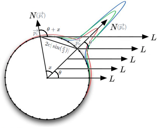
Let D(θ,c)=∫R2RN(∥pi−po∥)(cosθi)+dpi
where θ is the angle between the normal N of the center
position po and
the opposite direction L of the directional
light, and c is the curvature which can be calculated
on-the-fly as c1=ddx(P)ddx(N). However, the curvature is
precomputed by GFSDK_FaceWorks_CalculateMeshCurvature
in NVIDIA FaceWorks. Perhaps the on-the-fly method is NOT precise enough.
Diffusion Profile
The diffusion profile, which is approximated by the Gaussians, by [dEon 2007] is still used by EvaluateDiffusionProfile
in NVIDIA FaceWorks. However, the motivation of [dEon 2007] is to replace the general 2D convolution into two 1D
convolutions to improve the performance by using the Separable Filter property of the Gaussian Blur. But the D(θ,c) is pre-integrated offline by [Penner 2011 B], the
efficiency of the convolution is NOT important any more, and thus the more physically plausible diffusion profile
RN(r)=8πrS(e−Sr+e−31Sr) by [Christensen 2015] should be used.
Integrate on the Ring
By [Penner 2011 B], D(θ,c) is approximated as ∫−ππRN(2c∣sin(2x)∣)dx∫−ππRN(2c∣sin(2x)∣)(cos(θ+x))+dx and pre-integrated offline to be
stored in the LUT (Look Up Table).
However, this approximation can be improved much further.
Evidently, we have r=2c∣sin(2x)∣ and dxdr=2c21cos(2x)=ccos(2x) due
to the symmetry.
By "13.5.2 Polar Coordinates" of PBR
Book, we have that D(θ,c)=∫R2RN(∥pi−po∥)(cosθi)+dpi=∫0∞∫02πRN(r)r(cosθi)+dθrdr=∫0∞2πRN(r)r(cosθi)+dr=∫02c2πRN(r)r(cosθi)+dr+∫2c∞2πRN(r)r(cosθi)+dr. Note that θr is the polar coordinate which is not marked in the figure and is reduced due to the circular symmetry.
By "Figure 15.10" of PBR
Book, the diffusion profile falls off fairly quickly and the vicinal position pi,
which is too far away from the center position po, can
be ignored. This means that we have D(θ,c)=∫02c2πRN(r)r(cosθi)+dr+∫2c∞2πRN(r)r(cosθi)+dr≈∫02c2πRN(r)rdr∫02c2πRN(r)r(cosθi)+dr.
Evidently, the denominator does NOT equal one, since 1=∫R2RN(∥pi−po∥)dpi=∫02c2πRN(r)rdr+∫2c∞2πRN(r)rdr⇒∫02c2πRN(r)rdr=1−∫2c∞2πRN(r)rdr<1.
By Integration by Substitution
and symmetry, we have D(θ,c)=∫02c2πRN(r)rdr∫02c2πRN(r)r(cosθi)+dr=21∫−ππ2πRN(2c∣sin(2x)∣)(2c∣sin(2x)∣)dxdrdx21∫−ππ2πRN(2c∣sin(2x)∣)(2c∣sin(2x)∣)(cos(θ+x))+dxdrdx=21∫−ππ2πRN(2c∣sin(2x)∣)(2c∣sin(2x)∣)(ccos(2x))dx21∫−ππ2πRN(2c∣sin(2x)∣)(2c∣sin(2x)∣)(cos(θ+x))+(ccos(2x))dx.
Here is the MATLAB code which verifies D(θ,c)=21∫−ππ2πRN(2c∣sin(2x)∣)(2c∣sin(2x)∣)(ccos(2x))dx21∫−ππ2πRN(2c∣sin(2x)∣)(2c∣sin(2x)∣)(cos(θ+x))+(ccos(2x))dx.
global S = (1.0 / 0.7568628);
global c = 3.0;
global theta = pi / 4.0;
% ========================================================% numerator polar% ========================================================functiony = numerator_polar_positive(r)global S
global c
global theta
R_N_mul_r = (S / (8.0 * pi)) * (exp(-S * r) + exp(-(1.0 / 3.0) * S * r));
x = 2.0 * asin(r / (2.0 * c));
cos_theta_add_x = max(0.0, cos(theta + x));
y = 2.0 * pi * R_N_mul_r * cos_theta_add_x;
endfunction
functiony = numerator_polar_negative(r)global S
global c
global theta
R_N_mul_r = (S / (8.0 * pi)) * (exp(-S * r) + exp(-(1.0 / 3.0) * S * r));
x = -2.0 * asin(r / (2.0 * c));
cos_theta_add_x = max(0.0, cos(theta + x));
y = 2.0 * pi * R_N_mul_r * cos_theta_add_x;
endfunction
q_numerator_polar = 0.5 * (quad("numerator_polar_positive", 0, 2.0 * c) + quad("numerator_polar_negative", 0, 2.0 * c));
% output: "numerator_polar: 0.563473"
printf("numerator_polar: %f\n", q_numerator_polar);
% ========================================================% numerator ring% ========================================================functiony = numerator_ring(x)global S
global c
global theta
r = 2.0 * c * abs(sin(0.5 * x));
R_N_mul_r = (S / (8.0 * pi)) * (exp(-1.0 * S * r) + exp(-(1.0 / 3.0) * S * r));
cos_theta_add_x = max(0.0, cos(theta + x));
dr_per_dx = 2.0 * c * 0.5 * cos(0.5 * x);
y = 2.0 * pi * R_N_mul_r * cos_theta_add_x * dr_per_dx;
endfunction
q_numerator_ring = 0.5 * quad("numerator_ring", -pi, pi);
% output: "numerator_ring: 0.563473"
printf("numerator_ring: %f\n", q_numerator_ring);
% ========================================================% denominator polar% ========================================================functiony = denominator_polar(r)global S
R_N_mul_r = (S / (8.0 * pi)) * (exp(-S * r) + exp(-(1.0 / 3.0) * S * r));
y = 2.0 * pi * R_N_mul_r;
endfunction
q_denominator_polar = quad("denominator_polar", 0, 2.0 * c);
% output: "denominator_polar: 0.946522"
printf("denominator_polar: %f\n", q_denominator_polar);
% ========================================================% denominator ring% ========================================================functiony = denominator_ring(x)global S
global c
r = 2.0 * c * abs(sin(0.5 * x));
R_N_mul_r = (S / (8.0 * pi)) * (exp(-1.0 * S * r) + exp(-(1.0 / 3.0) * S * r));
dr_per_dx = 2.0 * c * 0.5 * cos(0.5 * x);
y = 2.0 * pi * R_N_mul_r * dr_per_dx;
endfunction
q_denominator_ring = 0.5 * quad("denominator_ring", -pi, pi);
% output: "denominator_ring: 0.946522"
printf("denominator_ring: %f\n", q_denominator_ring);
By [Penner 2011 A], three different normals should be used for different RGB channels and the LUT
should be sampled three times according to the three different θs.
Evidently, it is NOT efficient to sample the LUT three times and the N⋅L, which denotes the
part of the integral where x is close to zero and the diffuse profile is close to the peak, is detached from the
total integral D(θ,c) in NVIDIA FaceWorks.
However, the remaining part of the integral is relatively small, and thus FaceWorks maps the remaining
part of the integral from [-0.25, 0.25] to [0, 1] to fully use the precision of the texture (the rgbAdjust in the GFSDK_FaceWorks_GenerateCurvatureLUT
in NVIDIA FaceWorks).
The GFSDK_FaceWorks_EvaluateSSSDirectLight
is used to calculate the subsurface scattering on-the-fly. The LUT is only sampled once and three normals are used
to calculate the N⋅L which is detached
from the total integral.
Note that the demo of [Jimenez 2012] is provided by [Jimenez 2015]. Perhaps you can not believe it but
it is really the truth. The demo provided by [Jimenez 2015] has nothing to do with [Jimenez 2015].
This is really arcane, and I do spend some time to realize this fact.
The main idea of the Separable SSS is to approximate the diffusion profile kernel by the separable
kernel. Evidently, the Monte Carlo method is much more popular than the separable kernel in real
time rendering. Thus, the Separable SSS has been obsolete and should be replaced by the Disney SSS.
Note that the word "separable" in the "Separable SSS" has nothing to do with the
"11.4.1 Separable BSSRDFs" of PBR Book.
Separable Kernel
The approach of [dEon 2007] is to approximate the diffusion profile by the weighted sum of 6
Gaussians, and thus the general 2D convolution can be replaced by 12(2 x 6) 1D convolutions since the Gaussian blur is a separable filter. However, the approach proposed by
[dEon 2007] is applied in texture space which is too weird according to the convention of the real time rendering.
And the screen space approach is proposed by [Jimenez 2009]. However, the approach proposed by [Jimenez 2009]
still needs 12(2 x 6) passes to perform the 12(2 x 6) 1D convolutions. Evidently, this is still too expensive for
real time rendering. And thus, the 2 passes approach is proposed by [Jimenez 2012].
The main idea of [Jimenez 2012] is that in real time rendering, the non-separable diffusion profile is
represented by the discretized kernel where the SVD can be applied, and the SVD indicates that the diffusion
profile kernel can be approximated by a separable kernel M(xo,yo)=y∑(x∑E(xo+Δx,yo+Δy)⋅S(Δx))⋅ST(Δy) where
S(Δx)=R(0.001+falloffΔx⋅width)⋅strength+δ(Δx)⋅(1−strength) where R denotes the 1D diffusion
profile and δ(Δx) denotes the Delta Function such that δ(0)=1.
By [dEon 2007], the range of the significant contribution domain of the diffusion profile is about 16
mm. However, perhaps the diffusion profile is made narrower by the falloff in the formula by
[Jimenez 2012], and thus the range of the significant contribution domain of the diffusion profile is reduced to
6(3x2) mm (the RANGE in the calculateKernel
in Demo of [Jimenez 2015].
According to the numerical quadrature, the function value sampled from the separable
kernel S(Δx) should be
multiplied by the difference of the domain the Δx and the Δy (the area in the calculateKernel
in Demo of [Jimenez 2015]. And in Demo of [Jimenez 2015], it is manifested that the position of the sampling is
fixed, and the offset in mm between the vicinal position pi and
the center position po in
world space is stored in the w component of
the kernel member
of the SeparableSSS
class.
Technically, the position of the sampling is fixed. However, the SSSS_STRENGTH_SOURCE in Demo
of [Jimenez 2015] provides the scaling to tweak the offset. The SSSS_STRENGTH_SOURCE is
merely the alpha channel of the albedo texture, and is used to skip the pixels which do NOT represent the skin
(such as eyebrow). Evidently, the SSSS_STRENGTH_SOURCE has
nothing to do with the strength in the formula by [Jimenez 2012] at all. However, this empirical
value is adopted by both UE4 and Unity3D. The equivalent is called Opacity
Map in UE4 and Subsurface
Mask Map in Unity3D.
World Scale
Since the offset of position of the sampling is fixed and stored in the w component of
the kernel, the
mere purpose of the SSSSBlurPS is to transform
the offset from world space to texture space. Assuming that the center position is at the origin of the Y axis,
the transformation can be calculated as TextureSpace=21×tan(FOVY×0.5)1×ViewPositionZInWorldSpaceUnit1×1000×MetersPerWorldSpaceUnit1×WorldSpaceDeltaXInMM where the 1000 is to
transform from mm to m, the tan(FOVY×0.5)1 is the second row and the second
column of the projection matrix, and the 2 is to transform from NDC to texture space.
And since the 0.001+falloffΔx is passed to the diffusion
profile R(r) directly
in the calculateKernel
without the width in the formula by [Jimenez 2012] multiplied at all, the sssWidth in Demo of
[Jimenez 2015] can NOT be considered as the width in the formula by [Jimenez 2012].
In SSSSBlurPS,
the transformation is calculated as TextureSpace=tan(FOVY×0.5)1×ViewPositionZInWorldSpaceUnit1×3sssWidth×WorldSpaceDeltaXInMM. By comparing these two
formulas, a hypothesis can be proposed that MetersPerWorldSpaceUnit=1000×2×sssWidth3. The default of the sssWidth in Demo of
[Jimenez 2015] is 0.012, and thus the hypothesis implies that the MetersPerWorldSpaceUnit in Demo
of [Jimenez 2015] is 81. Fortunately, the vertex data of
the head mesh in the Demo of [Jimenez 2015] is consistent with this result that MetersPerWorldSpaceUnit=81.
Properties between Demo of [Jimenez 2015] and UE4
Name in Formula by [Jimenez 2012]
Demo of [Jimenez 2015]
Demo of [Jimenez 2015] Unity3D Default
UE4 Name
UE4 Default
strength
SSS Strength
(0.48, 0.41, 0.28)
Subsurface Color
(0.48, 0.41, 0.28)
falloff
SSS Falloff
(1.0, 0.37, 0.3)
Falloff Color
(1.0, 0.37, 0.3)
width
N/A
1
N/A
1
N/A
SSS Width
0.012 (0.125 Meters Per Unit)
World Unit Scale
0.1 (Units Per Centimeter)
strength
The strength is to lerp between the SSS diffuse term R(0.001+falloffΔx⋅width)
and the conventional diffuse term δ(Δx). Evidently,
when the strength equals 0, since S(Δx)=δ(Δx) and δ(0)=1, the formula is reduced to the conventional diffuse term M(xo,yo)=y∑(x∑E(xo+Δx,yo+Δy)⋅S(Δx))⋅ST(Δy)=y∑(x∑E(xo+Δx,yo+Δy)⋅δ(Δx))⋅δ(Δy)=E(xo,yo).
However, the SSSS_STRENGTH_SOURCE has
nothing to do with the strength in the formula by [Jimenez 2012] at all. The SSSS_STRENGTH_SOURCE is
merely the alpha channel of the albedo texture, and is used to skip the pixels which do NOT represent the skin
(such as eyebrow). this empirical value is adopted by both UE4 and Unity3D. The equivalent is called Opacity
Map in UE4 and Subsurface
Mask Map in Unity3D.
width
The 0.001+falloffΔx is passed to the diffusion
profile R(r)
directly in the calculateKernel
without the width in the formula by [Jimenez 2012] multiplied at all. This implies the
width in the formula by [Jimenez 2012] is actually fixed at 1.
The main idea of the Disney SSS is to use the Monte Carlo method to integrate Lo(po,ωo)=∫R2R(∥pi−po∥)F(pi,ωo)dpi in
real time.
By [Christensen 2015], the diffusion profile R(r)=8πrAS(e−Sr+e−31Sr), where the A is the surface albedo and the S is the
scaling factor, is used. The derivation of the diffusion profile will NOT be involved here, but you can refer to
"15.5 Subsurface Scattering Using the Diffusion Equation" of PBR
Book V3 for more information.
4-3-1. Monte Carlo Integration
PDF
By [Christensen 2015], we have the norm of the diffusion profile ∫o∞R(r)2πrdr=A. This means that the surface albedo A is
exactly the total diffuse reflectance and we have the normalized diffusion profile RN(r)=AR(r). And by [Golubev 2018], the
normalized function p(r,θ)=AR(r)r=RN(r)r=8πs(e−sr+e−3sr) is used as the PDF.
Estimator
By appealing p(r,θ)=RN(r)r to Lo(po,ωo)=∫R2RN(∥pi−po∥)Rd(pi)F(pi,ωo)dpi, we
have Lo(po,ωo)=∫R2RN(∥pi−po∥)Rd(pi)F(pi,ωo)dpi=∫0∞∫02πRN(r)Rd(pi)F(p)rdθdr=∫0∞∫02πrp(r,θ)Rd(pi)F(p)rdθdr=∫0∞∫02πp(r,θ)Rd(pi)F(p)dθdr.
By "Equation (13.3)" of PBR Book, we have
Lo(po,ωo)=∫0∞∫02πp(r,θ)Rd(pi)F(p)dθdr=∑N1pi(r,θ)p(r,θ)Rd(pi)F(p).
Technically, RN(r) is spectrally varying since the scaling factor s is
spectrally varying. This means that the p(r,θ)=RN(r)r is a vector "RGB". However,
the PDF, which is used to calculate the sampling of the diffusion profile, should be a scalar "float".
Thus, the spectral channel i is selected as the PDF and we have pi(r,θ)=ARi(r)r. This means that the p(r,θ) in the
numerator is a vector "RGB" while the pi(r,θ) in the denominator is a scalar "float".
Analogously to the "Equation 15.11" of PBR
Book, the average over all spectral channels can be used as the PDF. However, in real time rendering, the
spectral channel corresponding to the minimum PDF is usually used for efficiency.
Sampling 2D Diffusion Profile
Analogously to "Equation (14.1)" of PBR
Book, we can derive the sampling of diffusion profile. Since the diffusion profile is isotropic (radially
symmetric), we have p(θ∣r)=2π1⇒θ=2πξ2. Since the PDF is p(r,θ)=AR(r)r, we have the marginal PDF p(r)=∫02πR(r)dθ=R(r)2πr and the CDF P(r)=∫0rp(r′)dr′=ξ1. Fortunately, by [Golubev 2018], the inverse of the CDF is closed-form and we have r=s1⋅3⋅log2(4u1+G(u)−31+G(u)31)
where G(u)=1+4u(2u+1+4u2) and u=1−ξ1.
By "20.3 Quasirandom Low-Discrepancy Sequences" of [Colbert 2007] and "13.8.2 Quasi
Monte Carlo" of PBR
Book, the low-discrepancy sequence is the better alternative than pseudo-random
sequence to generate the ξ1 and ξ2.
For example, the Hammersley sequence ("7.4.1 Hammersley and Halton
Sequences" of PBR
Book) is a typical low-discrepancy sequence.
In UE4, the Center Sample Reweighting, which is controlled by the macro
REWEIGHT_CENTER_SAMPLE, is used, and the CDF of the center sample is calculated
and removed from the vicinal samples. And UE4 claims that the result of this approach is still unbiased.
Sampling 3D Surface
By "Figure 15.8" of PBR
Book, the sampling of the 2D diffusion profile should be mapped to the position on the 3D surface. And by
"Figure 15.12" of PBR
Book, the radii under three projection axes, which are the three basis vectors of the tangent space at the
center position po, are
calculated. Evidently, it is too inefficient to be used in real time rendering.
Analogously to the the "Bilateral Filter" by [Mikkelsen 2010], the radius is approximated as
∥pixy−poxy∥2+Δxz2 by [Golubev 2018]. The Bilateral Filter is controlled by the macro
SSS_BILATERAL_FILTER in Unity3D and the macro USE_BILATERAL_FILTERING in UE4.
The Stretch Texture by "Correcting for UV Distortion" of [dEon 2007] can be
used to calculate the radius as well. However, it is too inefficient to be used in real time rendering.
By "11.1.3 Out-Scattering and Attenuation" of PBR
Book, we have the mean free pathστ1=σa+σs1 where στ
is the extinction coefficient, σa
is the absorption coefficient and σs
is the scattering coefficient.
Note that, in UE4, the scaling factor s is calculated by S=MeanFreePathColor⋅MeanFreePathDistanceGetScalingFactor(SurfaceAlbedo) where the GetScalingFactor follows the Equation 5, 6,
7 of [Christensen 2015]. But, by [Christensen 2015], the result of the GetScalingFactor is exactly the scaling
factor. Thus, the denominator is NOT reasonable.
5. Transmittance
The blur pass is only to accumulate the vicinal position pi which
is on the same face as the center position po. And
the transmittance is to accumulate the vicinal position pi which
is on the different face from the center position po.
5-1. Thickness Map
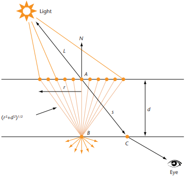
By "16.3 Simulating Absorption Using Depth Maps" of [Green 2004], if the objects are assumed
to be convex, the thickness (the distance a light ray travels inside an object) can be estimated by using the shadow
maps.
However, the transmittance coefficient by the Beer–Lambert law is too inaccurate to be used.
By [Jimenez 2010], the transmittance coefficient can be calculated based on the diffusion profile rather
than the Beer–Lambert law. The idea of the "14.5.3 Modified Translucent Shadow Maps" of [dEon 2007] is
applied. By assuming that the form factors F(pi,ωo) are the same, by "13.5.2 Polar Coordinates" of
PBR
Book, the transmittance coefficient can be calculated as Lo(po,ωo)=∫R2R(∥pi−po∥)F(pi,ωo)dpi=F∫R2R(∥pi−po∥)dpi=F∫o∞2πrR(r2+d2)dr⇒T(d)=∫o∞2πrR(r2+d2)dr where d is the thickness, r is the
distance on the different face of the surface and R(r2+d2) is the diffusion profile.
Usually, the form factor is approximated by the Lambert BRDF and the light is assumed to be the
directional light. The Delta
Distribution is applied and we have F=π1EL(cosθi)+. Evidently, the (cosθi)+ varies at each position. However, since the form factors are assumed to be the same, the maximum value of (cosθi)+ is used. This means that we have F=π1EL(cosθi)+≈π1EL(1)+=π1EL.
By [Golubev 2018], the diffuse profile of [Christensen 2015] is applied, and we have T(d)=∫0∞2πr⋅R(r2+d2)dr=41A(e−sd+3e−3sd).
The transmittance coefficient by [Golubev 2018] is calculated by the ComputeTransmittanceDisney
in Unity3D.
6. Specular BRDF
6-1. Two-lobe Blinn-Phong
The Two-lobe Blinn-Phong is calculated by EvaluateSpecularLight
in NVIDIA FaceWorks.
TODO
6-2. Dual Trowbridge-Reitz
The Dual Trowbridge-Reitz is calculated by DualSpecularGGX
in UE4.