Volume Rendering
Rendering Equation
Notation
Description
Shader Code Convention
p
→
\displaystyle \overrightarrow{p}
p
Shading Position
N/A
ω
o
→
\displaystyle \overrightarrow{\omega_o}
ω o
Outgoing Direction
V
L
o
(
p
→
,
ω
i
→
)
\displaystyle
\operatorname{L_o}(\overrightarrow{p}, \overrightarrow{\omega_i})
L o ( p
, ω i
)
Outgoing Radiance
N/A
L
e
(
p
→
,
ω
o
→
)
\displaystyle
\operatorname{L_e}(\overrightarrow{p}, \overrightarrow{\omega_o})
L e ( p
, ω o
)
Emissive Radiance
N/A
ω
i
→
\displaystyle \overrightarrow{\omega_i}
ω i
Incident Direction
L
f
(
p
→
,
ω
i
→
,
ω
o
→
)
\displaystyle
\operatorname{f}(\overrightarrow{p}, \overrightarrow{\omega_i},
\overrightarrow{\omega_o})
f ( p
, ω i
, ω o
)
BRDF
N/A
L
i
(
p
→
,
ω
i
→
)
\displaystyle
\operatorname{L_i}(\overrightarrow{p}, \overrightarrow{\omega_i})
L i ( p
, ω i
)
Incident Radiance
N/A
(
cos
θ
i
)
+
\displaystyle (\cos \theta_i)^+
( cos θ i ) +
N/A
clamp(dot(N, L), 0.0, 1.0)
r
(
p
→
,
ω
i
→
)
\displaystyle
\operatorname{r}(\overrightarrow{p}, \overrightarrow{\omega_i})
r ( p
, ω i
)
Ray-Casting Function
N/A
The Rendering Equation is also called the LTE (Light
Transport Equation ) by "14.4 The Light Transport Equation" of PBR
Book V3 . And we have the Rendering Equation
L
o
(
p
→
,
ω
o
→
)
=
L
e
(
p
→
,
ω
o
→
)
+
∫
Ω
f
(
p
→
,
ω
i
→
,
ω
o
→
)
L
i
(
p
→
,
ω
i
→
)
(
cos
θ
i
)
+
d
ω
i
→
\displaystyle
\operatorname{L_o}(\overrightarrow{p}, \overrightarrow{\omega_o}) =
\operatorname{L_e}(\overrightarrow{p}, \overrightarrow{\omega_o}) + \int_\Omega
\operatorname{f}(\overrightarrow{p}, \overrightarrow{\omega_i},
\overrightarrow{\omega_o}) \operatorname{L_i}(\overrightarrow{p},
\overrightarrow{\omega_i}) (\cos \theta_i)^+ \, d \overrightarrow{\omega_i}
L o ( p
, ω o
) = L e ( p
, ω o
) + ∫ Ω f ( p
, ω i
, ω o
) L i ( p
, ω i
) ( cos θ i ) + d ω i
According to the Rendering Equation , by OSL (Open Shading Language) , the
surface and the light are actually the same thing, since the light is merely the surface which is emissive.
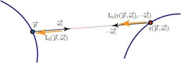
By "Figure 11.1" of Real-Time Rendering Fourth
Edition and "Figure 14.14" of PBR
Book V3 , by assuming no participating media , we have the relationship
L
i
(
p
→
,
ω
i
→
)
=
L
o
(
r
(
p
→
,
ω
i
→
)
,
−
ω
i
→
)
\displaystyle
\operatorname{L_i}(\overrightarrow{p}, \overrightarrow{\omega_i}) =
\operatorname{L_o}(\operatorname{r}(\overrightarrow{p}, \overrightarrow{\omega_i}),
-\overrightarrow{\omega_i})
L i ( p
, ω i
) = L o ( r ( p
, ω i
) , − ω i
)
r
(
p
→
,
ω
→
)
\displaystyle \operatorname{r}(\overrightarrow{p},
\overrightarrow{\omega})
r ( p
, ω
)
L
i
(
p
→
,
ω
i
→
)
\displaystyle
\operatorname{L_i}(\overrightarrow{p}, \overrightarrow{\omega_i})
L i ( p
, ω i
)
L
o
(
r
(
p
→
,
ω
i
→
)
,
−
ω
i
→
)
\displaystyle
\operatorname{L_o}(\operatorname{r}(\overrightarrow{p}, \overrightarrow{\omega_i}),
-\overrightarrow{\omega_i})
L o ( r ( p
, ω i
) , − ω i
)
r
(
p
→
,
ω
i
→
)
\displaystyle \operatorname{r}(\overrightarrow{p},
\overrightarrow{\omega_i})
r ( p
, ω i
)
Hence, both the incident radiance
L
i
(
p
→
,
ω
→
)
\displaystyle
\operatorname{L_i}(\overrightarrow{p}, \overrightarrow{\omega})
L i ( p
, ω
)
L
o
(
p
→
,
ω
→
)
\displaystyle
\operatorname{L_o}(\overrightarrow{p}, \overrightarrow{\omega})
L o ( p
, ω
)
L
(
p
→
,
ω
→
)
\displaystyle \operatorname{L}(\overrightarrow{p},
\overrightarrow{\omega})
L ( p
, ω
)
L
(
p
→
,
ω
o
→
)
=
L
e
(
p
→
,
ω
o
→
)
+
∫
Ω
f
(
p
→
,
ω
i
→
,
ω
o
→
)
L
(
r
(
p
→
,
ω
i
→
)
,
−
ω
i
→
)
(
cos
θ
i
)
+
d
ω
i
→
\displaystyle \operatorname{L}(\overrightarrow{p},
\overrightarrow{\omega_o}) = \operatorname{L_e}(\overrightarrow{p},
\overrightarrow{\omega_o}) + \int_\Omega \operatorname{f}(\overrightarrow{p},
\overrightarrow{\omega_i}, \overrightarrow{\omega_o})
\operatorname{L}(\operatorname{r}(\overrightarrow{p}, \overrightarrow{\omega_i}),
-\overrightarrow{\omega_i}) (\cos \theta_i)^+ \, d \overrightarrow{\omega_i}
L ( p
, ω o
) = L e ( p
, ω o
) + ∫ Ω f ( p
, ω i
, ω o
) L ( r ( p
, ω i
) , − ω i
) ( cos θ i ) + d ω i
L
(
p
→
,
ω
→
)
\displaystyle \operatorname{L}(\overrightarrow{p},
\overrightarrow{\omega})
L ( p
, ω
)
By "Light transport and the rendering equation" of CS 348B - Computer Graphics: Image Synthesis
Techniques and "Global Illumination and Rendering Equation" of CS 294-13 Advanced Computer Graphics , this
differential equation is actually the Fredholm Integral Equation of which the
solution is the Liouville–Neumann
Series . And thus, the solution of this differential equation can be written as the recursive form
L
=
E
+
KE
+
K
2
E
+
K
3
E
+
…
\text{L} = \text{E} + \text{K}\text{E} +
{\text{K}}^2\text{E} + {\text{K}}^3\text{E} + \ldots
L = E + K E + K 2 E + K 3 E + … .
Radiative Transfer Equation
Notation
Description
Shader Code Convention
σ
t
(
p
→
+
ω
i
→
t
,
ω
i
→
)
\displaystyle
\operatorname{\sigma_t}(\overrightarrow{p} + \overrightarrow{\omega_i}t,
\overrightarrow{\omega_i})
σ t ( p
+ ω i
t , ω i
)
Attenuation/Extinction Coefficient
N/A
σ
a
(
p
→
+
ω
i
→
t
,
ω
i
→
)
\displaystyle
\operatorname{\sigma_a}(\overrightarrow{p} + \overrightarrow{\omega_i}t,
\overrightarrow{\omega_i})
σ a ( p
+ ω i
t , ω i
)
Absorption Coefficient
N/A
σ
s
(
p
→
+
ω
i
→
t
,
ω
i
→
)
\displaystyle
\operatorname{\sigma_s}(\overrightarrow{p} + \overrightarrow{\omega_i}t,
\overrightarrow{\omega_i})
σ s ( p
+ ω i
t , ω i
)
Scattering Coefficient
N/A
T
τ
(
p
→
,
ω
i
→
,
t
)
\displaystyle
\operatorname{\Tau_{\tau}}(\overrightarrow{p}, \overrightarrow{\omega_i}, t)
T τ ( p
, ω i
, t )
Multiplicative Transmittance
N/A
p
(
p
→
+
ω
i
→
t
,
ω
i
→
,
ω
s
→
)
\displaystyle
\operatorname{p}(\overrightarrow{p} + \overrightarrow{\omega_i}t,
\overrightarrow{\omega_i}, \overrightarrow{\omega_s})
p ( p
+ ω i
t , ω i
, ω s
)
Phase Function
N/A
The RTE (Radiative Transfer Equation ) is also called the
complete transport equation by "Participating media" of CS 348B - Computer Graphics: Image Synthesis
Techniques , and is also called the Equation of Transfer by "15.1 The Equation of
Transfer" of PBR Book
V3 .
By "Participating media" of CS
348B - Computer Graphics: Image Synthesis Techniques , [Fong 2017], "Figure 14.3" of Real-Time Rendering Fourth Edition and "15.1 The Equation
of Transfer" of PBR Book
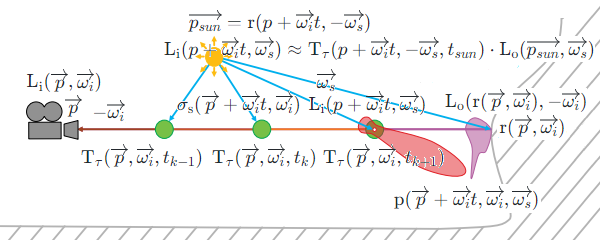
V3 , we have the RTE (Radiative Transfer Equation )
L
i
(
p
→
,
ω
i
→
)
=
∫
0
t
r
T
τ
(
p
→
,
ω
i
→
,
t
)
⋅
(
L
e
(
p
→
+
ω
i
→
t
,
ω
i
→
)
+
σ
s
(
p
→
+
ω
i
→
t
,
ω
i
→
)
(
∫
Ω
p
(
p
→
+
ω
i
→
t
,
ω
i
→
,
ω
s
→
)
L
i
(
p
+
ω
i
→
t
,
ω
s
→
)
d
ω
s
→
)
)
d
t
+
T
τ
(
p
→
,
ω
i
→
,
t
r
)
⋅
L
o
(
r
(
p
→
,
ω
i
→
)
,
−
ω
i
→
)
\displaystyle
\operatorname{L_i}(\overrightarrow{p}, \overrightarrow{\omega_i}) = \int_0^{t_r}
\operatorname{\Tau_{\tau}}(\overrightarrow{p}, \overrightarrow{\omega_i}, t) \cdot
\left\lparen \operatorname{L_e}(\overrightarrow{p} + \overrightarrow{\omega_i}t,
\overrightarrow{\omega_i}) + \operatorname{\sigma_s}(\overrightarrow{p} +
\overrightarrow{\omega_i}t, \overrightarrow{\omega_i}) \left\lparen \int_{\Omega}
\operatorname{p}(\overrightarrow{p} + \overrightarrow{\omega_i}t,
\overrightarrow{\omega_i}, \overrightarrow{\omega_{s}}) \operatorname{L_i}(p +
\overrightarrow{\omega_i}t, \overrightarrow{\omega_{s}}) \, d
\overrightarrow{\omega_{s}} \right\rparen \right\rparen \, dt +
\operatorname{\Tau_{\tau}}(\overrightarrow{p}, \overrightarrow{\omega_i}, t_r) \cdot
\operatorname{L_o}(\operatorname{r}(\overrightarrow{p}, \overrightarrow{\omega_i}),
-\overrightarrow{\omega_i})
L i ( p
, ω i
) = ∫ 0 t r T τ ( p
, ω i
, t ) ⋅ ( L e ( p
+ ω i
t , ω i
) + σ s ( p
+ ω i
t , ω i
) ( ∫ Ω p ( p
+ ω i
t , ω i
, ω s
) L i ( p + ω i
t , ω s
) d ω s
) ) d t + T τ ( p
, ω i
, t r ) ⋅ L o ( r ( p
, ω i
) , − ω i
)
r
(
p
→
,
ω
i
→
)
\displaystyle \operatorname{r}(\overrightarrow{p},
\overrightarrow{\omega_i})
r ( p
, ω i
)
t
r
\displaystyle t_r
t r
(
p
→
+
ω
i
→
t
r
)
=
r
(
p
→
,
ω
i
→
)
\displaystyle (\overrightarrow{p} +
\overrightarrow{\omega_i} t_r) = \operatorname{r}(\overrightarrow{p},
\overrightarrow{\omega_i})
( p
+ ω i
t r ) = r ( p
, ω i
)
T
τ
(
p
→
,
ω
i
→
,
t
)
=
e
−
τ
(
p
→
,
ω
i
→
,
t
)
\displaystyle
\operatorname{\Tau_{\tau}}(\overrightarrow{p}, \overrightarrow{\omega_i}, t) =
e^{-\operatorname{\tau}(\overrightarrow{p}, \overrightarrow{\omega_i}, t)}
T τ ( p
, ω i
, t ) = e − τ ( p
, ω i
, t ) multiplicative
transmittance where
τ
(
p
→
,
ω
i
→
,
t
)
=
∫
0
t
σ
t
(
p
→
+
ω
i
→
t
′
,
ω
i
→
)
d
t
′
\displaystyle
\operatorname{\tau}(\overrightarrow{p}, \overrightarrow{\omega_i}, t) = \int_0^t
\operatorname{\sigma_t}(\overrightarrow{p} + \overrightarrow{\omega_i}t',
\overrightarrow{\omega_i}) \, dt'
τ ( p
, ω i
, t ) = ∫ 0 t σ t ( p
+ ω i
t ′ , ω i
) d t ′ optical
thickness where
σ
t
(
p
→
+
ω
i
→
t
′
,
ω
i
→
)
=
σ
a
(
p
→
+
ω
i
→
t
′
,
ω
i
→
)
+
σ
s
(
p
→
+
ω
i
→
t
′
,
ω
i
→
)
\displaystyle
\operatorname{\sigma_t}(\overrightarrow{p} + \overrightarrow{\omega_i}t',
\overrightarrow{\omega_i}) = \operatorname{\sigma_a}(\overrightarrow{p} +
\overrightarrow{\omega_i}t', \overrightarrow{\omega_i}) +
\operatorname{\sigma_s}(\overrightarrow{p} + \overrightarrow{\omega_i}t',
\overrightarrow{\omega_i})
σ t ( p
+ ω i
t ′ , ω i
) = σ a ( p
+ ω i
t ′ , ω i
) + σ s ( p
+ ω i
t ′ , ω i
) attenuation/extinction
coefficient where
σ
a
\displaystyle \operatorname{\sigma_a}
σ a absorption
coefficient and
σ
s
\displaystyle \operatorname{\sigma_s}
σ s scattering
coefficient , and
p
(
p
→
+
ω
i
→
t
,
ω
i
→
,
ω
s
→
)
\displaystyle \operatorname{p}(\overrightarrow{p} +
\overrightarrow{\omega_i}t, \overrightarrow{\omega_i}, \overrightarrow{\omega_s})
p ( p
+ ω i
t , ω i
, ω s
) phase function .
Technically, the relationship between
L
i
(
p
+
ω
i
→
t
,
ω
s
→
)
\displaystyle \operatorname{L_i}(p +
\overrightarrow{\omega_i}t, \overrightarrow{\omega_{s}})
L i ( p + ω i
t , ω s
)
L
o
(
p
s
u
n
→
,
ω
s
→
)
\displaystyle
\operatorname{L_o}(\overrightarrow{p_{sun}}, \overrightarrow{\omega_{s}})
L o ( p s u n
, ω s
) RTE
(Radiative Transfer Equation ). However, in real time rendering, we assume that
L
i
(
p
+
ω
i
→
t
,
ω
s
→
)
≈
T
τ
(
p
+
ω
i
→
t
,
−
ω
s
→
,
t
s
u
n
)
⋅
L
o
(
p
s
u
n
→
,
ω
s
→
)
\displaystyle \operatorname{L_i}(p +
\overrightarrow{\omega_i}t, \overrightarrow{\omega_{s}}) \approx
\operatorname{\Tau_{\tau}}(p + \overrightarrow{\omega_i}t, -\overrightarrow{\omega_{s}},
t_{sun}) \cdot \operatorname{L_o}(\overrightarrow{p_{sun}}, \overrightarrow{\omega_{s}})
L i ( p + ω i
t , ω s
) ≈ T τ ( p + ω i
t , − ω s
, t s u n ) ⋅ L o ( p s u n
, ω s
)
p
s
u
n
→
=
r
(
p
+
ω
i
→
t
,
−
ω
s
→
)
\displaystyle \overrightarrow{p_{sun}} =
\operatorname{r}(p + \overrightarrow{\omega_i}t, -\overrightarrow{\omega_{s}})
p s u n
= r ( p + ω i
t , − ω s
)
L
o
(
p
s
u
n
→
,
ω
s
→
)
\displaystyle
\operatorname{L_o}(\overrightarrow{p_{sun}}, \overrightarrow{\omega_{s}})
L o ( p s u n
, ω s
)
∫
0
t
r
s
T
τ
(
p
+
ω
i
→
t
,
−
ω
s
→
,
t
s
)
⋅
(
L
e
(
p
+
ω
i
→
t
−
ω
s
→
t
s
,
−
ω
s
→
)
+
σ
s
(
p
+
ω
i
→
t
−
ω
s
→
t
s
,
−
ω
s
→
)
(
∫
Ω
p
(
p
+
ω
i
→
t
−
ω
s
→
t
s
,
−
ω
s
→
,
ω
p
→
)
L
i
(
p
+
ω
i
→
t
−
ω
s
→
t
s
,
ω
p
→
)
d
ω
p
→
)
)
d
t
s
\displaystyle \int_0^{t_r^s}
\operatorname{\Tau_{\tau}}(p + \overrightarrow{\omega_i}t, -\overrightarrow{\omega_{s}},
t_s) \cdot \left\lparen \operatorname{L_e}(p + \overrightarrow{\omega_i}t
-\overrightarrow{\omega_{s}}t_s, -\overrightarrow{\omega_{s}}) +
\operatorname{\sigma_s}(p + \overrightarrow{\omega_i}t -\overrightarrow{\omega_{s}}t_s,
-\overrightarrow{\omega_{s}}) \left\lparen \int_{\Omega} \operatorname{p}(p +
\overrightarrow{\omega_i}t -\overrightarrow{\omega_{s}}t_s,
-\overrightarrow{\omega_{s}}, \overrightarrow{\omega_{p}}) \operatorname{L_i}(p +
\overrightarrow{\omega_i}t -\overrightarrow{\omega_{s}}t_s, \overrightarrow{\omega_{p}})
\, d \overrightarrow{\omega_{p}} \right\rparen \right\rparen \, dt_s
∫ 0 t r s T τ ( p + ω i
t , − ω s
, t s ) ⋅ ( L e ( p + ω i
t − ω s
t s , − ω s
) + σ s ( p + ω i
t − ω s
t s , − ω s
) ( ∫ Ω p ( p + ω i
t − ω s
t s , − ω s
, ω p
) L i ( p + ω i
t − ω s
t s , ω p
) d ω p
) ) d t s
(
p
→
+
ω
i
→
t
−
ω
s
→
t
r
s
)
=
r
(
p
+
ω
i
→
t
,
−
ω
s
→
)
=
p
s
u
n
→
\displaystyle (\overrightarrow{p} +
\overrightarrow{\omega_i}t -\overrightarrow{\omega_{s}}t_r^s) = \operatorname{r}(p +
\overrightarrow{\omega_i}t, -\overrightarrow{\omega_{s}}) = \overrightarrow{p_{sun}}
( p
+ ω i
t − ω s
t r s ) = r ( p + ω i
t , − ω s
) = p s u n
RTE (Radiative Transfer Equation ) is ignored.
Evidently, the relationship
L
i
(
p
→
,
ω
i
→
)
=
L
o
(
r
(
p
→
,
ω
i
→
)
,
−
ω
i
→
)
\displaystyle
\operatorname{L_i}(\overrightarrow{p}, \overrightarrow{\omega_i}) =
\operatorname{L_o}(\operatorname{r}(\overrightarrow{p}, \overrightarrow{\omega_i}),
-\overrightarrow{\omega_i})
L i ( p
, ω i
) = L o ( r ( p
, ω i
) , − ω i
) Real-Time Rendering Fourth Edition and "Figure 14.14"
of PBR
Book V3 is the simplified case of the RTE (Radiative Transfer
Equation ) by assuming no participating media.
Epipolar Sampling
[Yusov 2013]
TODOhttps://www.intel.com/content/dam/develop/external/us/en/documents/gdc2013-lightscattering-final.pdf https://www.intel.com/content/dam/develop/external/us/en/documents/outdoor-light-scattering-update.pdf https://github.com/GameTechDev/OutdoorLightScattering
Tessellation
[Cantlay 2014]
TODOhttps://github.com/NVIDIAGameWorks/VolumetricLighting
References
[Yusov 2013] Egor Yusov.
"Practical Implementation of Light Scattering Effects Using Epipolar Sampling and 1D Min/Max Binary
Trees." GDC 2013 Iain
Cantlay. From Terrain to Godrays Better Use of DirectX11. GDC 2014. Sebastien
Hillaire. "Physically Based Sky, Atmosphere and Cloud Rendering in Frostbite." SIGGRAPH
2016. Nathan
Hoobler. "Fast, Flexible, Physically-Based Volumetric Light Scattering." GTC 2016. Julian Fong, Magnus Wrenninge, Christopher Kulla, Ralf
Habel. "Production Volume Rendering." SIGGRAPH 2017.