VXGI (Voxel Global Illumintaion)

1. Workflow

1-1. Photon Mapping

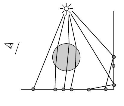
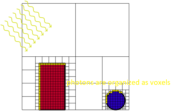
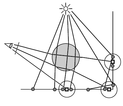
By "4.3 Overview" of [Jensen 2001] and "16.2.2 Photon Mapping" of PBR Book V3, the photon mapping is composed of two steps: photon tracing and rendering. During the photon tracing step, the photon rays are traced from the light sources, and the lighting information of the intersection positions of these photon rays is recorded as the photons. During the rendering step, the primary rays are traced from the camera and the final gather rays are traced from the final gather points, and the lighting information of the vicinal photons of the intersection positions of these primary rays or final gather rays is used to approximate the lighting of these intersection points by density estimation.

By "7.5 Photon Gathering" of [Jensen 2001], "38.2.2 Final Gathering" of [Hachisuka 2005] and "16.2.2 Photon Mapping" of PBR Book V3, the rendering step of the photon mapping is usually composed of two steps: radiance estimate and final gathering. 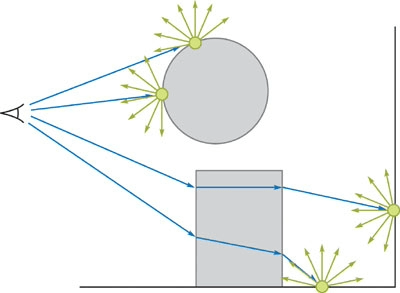During the radiance estimate step, the primary rays are traced from the camera, and the lighting information of the vicinal photons of the intersection positions of these primary rays is used to approximate the lighting of these intersection points by density estimation. During the final gathering step, from some of the intersection positions of the primary rays, which are called the final gather points, the final gather rays are traced, and the lighting information of the vicinal photons of the intersection positions of these final gather rays is used to approximate the lighting of these intersection positions by density estimation.

Photon Tracing	Rendering / Radiance-Estimate	Rendering / Final Gathering

1-2. VXGI (Voxel Global Illumintaion)

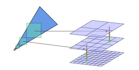
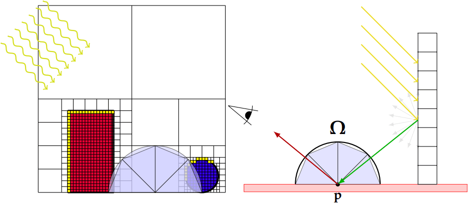
By [Crassin 2011], the VXGI (Voxel Global Illumintaion) is composed of four steps: voxelization, light injection, filtering and cone tracing. The idea of the VXGI is intrinsically to implement the photon mapping by storing the photons in the voxels. The light injection step of the VXGI is analogous to the photon tracing step of the photon mapping. The cone tracing of the VXGI is analogous to the rendering / final gathering step of the photon mapping. The filtering step of the VXGI is analogous to the idea of the density estimation of the photon mapping.

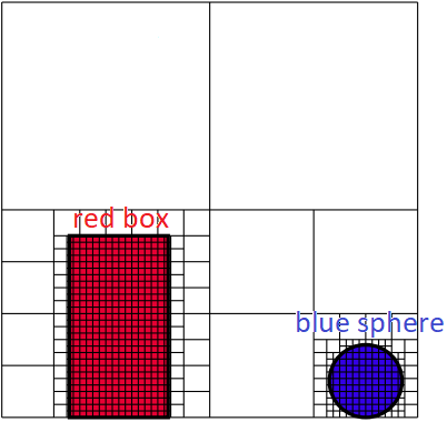
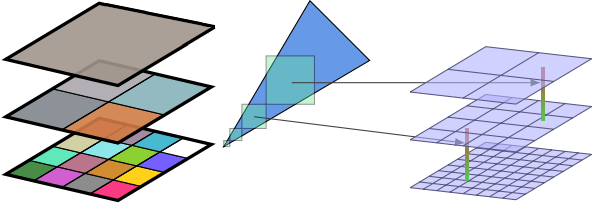
Voxelization	Light Injection	Filtering	Cone Tracing

2-1. Voxelization

Clipmap

TODO: by [McLaren 2015] and [Eric 2017], clipmap is better than SVO (sparse voxel octree).

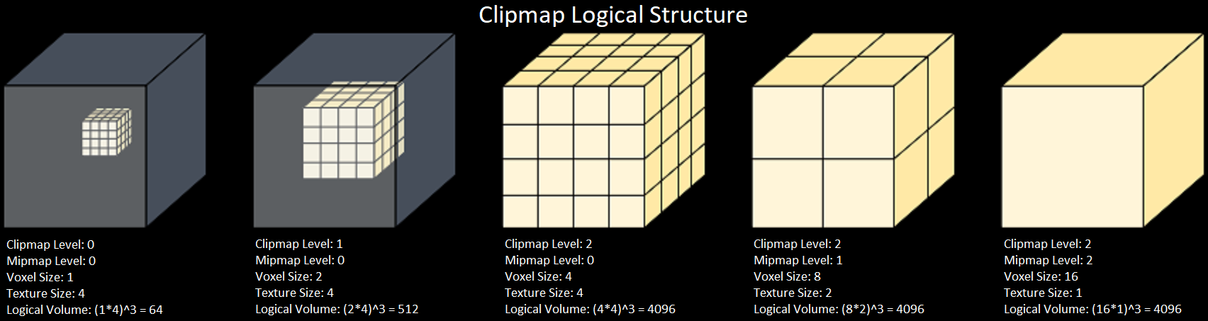
Clipmap Logical Structure

[Panteleev 2014]: "CLIPMAP VS. MIPMAP"

Texture size (for zeroth mipmap level) is the same for all clipmap levels, which is called that clipmap size
The voxel size increses
Only the last level has more than one mipmap levels (the logical volume remains the same within the same clipmap level)

NVIDIA VXGI Implementation:

Logical Structure:
clipmap level 0-3: only one mipmap level
clipmap level 4: mipmap 0-5 (6 levels)

Physical Structure:
Texture3D 128*128*785

MSAA

TODO: conservative rasterization
TODO: simulate "conservative rasterization" by MSAA ([Takeshige 2015])

2-2. Light Injection

TODO: not related to "ambient occlusion"

2-3. Filtering

TODO: anisotropic voxel

2-4. Cone Tracing

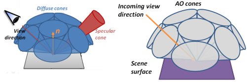
By Additive Interval Property, the ambient occlusion can be calculated as $\displaystyle \operatorname{k_A} = \int_\Omega \frac{1}{\pi} \operatorname{V}(\overrightarrow{\omega_i}) (\cos \theta_i)^+ \, d \overrightarrow{\omega_i} = \frac{1}{\pi} \sum_{i=0}^{n} \left\lparen \int_{\Omega_i} \operatorname{V}(\overrightarrow{\omega_i}) (\cos \theta_i)^+ \, d \overrightarrow{\omega_i} \right\rparen$ where n is the number of cones, and $\displaystyle \Omega_i$ is the solid angle subtended by the ith cone.

By [Crassin 2011 B], the visibility $\displaystyle \operatorname{V}(\overrightarrow{\omega_i})$ is assumed to be the same for all directions within the same cone, and the calculation of the ambient occlusion can be simplified as $\displaystyle \int_{\Omega_i} \operatorname{V}(\overrightarrow{\omega_i}) (\cos \theta_i)^+ \, d \overrightarrow{\omega_i} \approx \operatorname{V_c}(\Omega_i) \cdot \int_{\Omega_i} (\cos \theta_i)^+ \, d \overrightarrow{\omega_i}$ where $\displaystyle \operatorname{V_c}(\Omega_i) = 1 - \operatorname{A_{Final}}$ is the inverse of the final occlusion of the cone tracing.

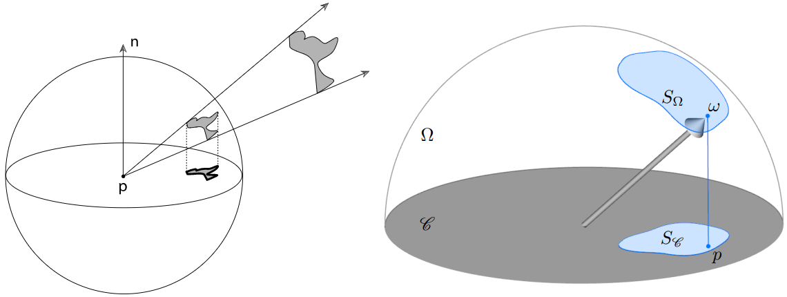
By "5.5.1 Integrals over Projected Solid Angle" of PBRT-V3 and [Heitz 2017], the integral of the clamped cosine $\displaystyle \int_{\Omega_i} (\cos \theta_i)^+ \, d \overrightarrow{\omega_i}$ can be calculated as the projected area on the unit disk.

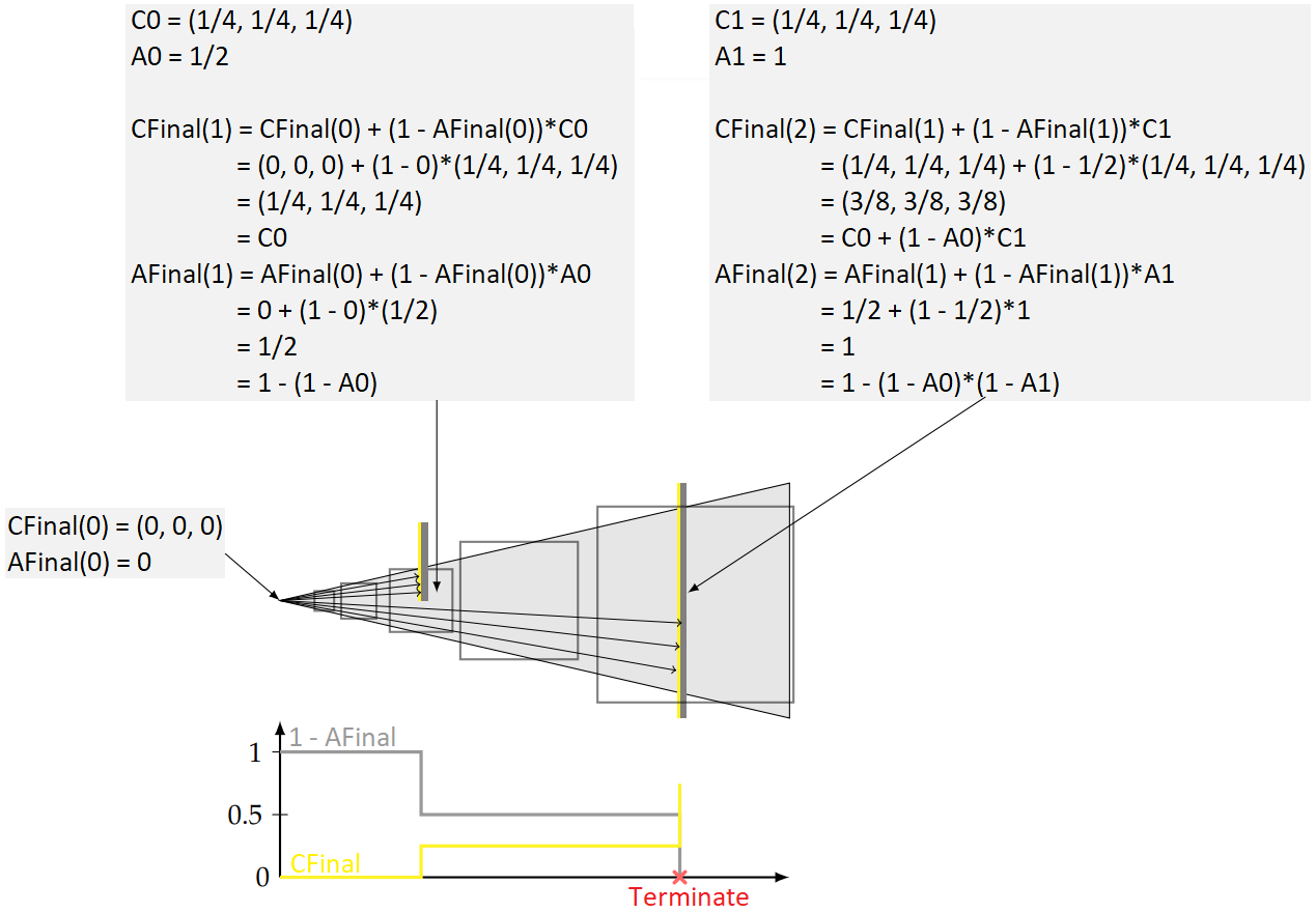
By [Crassin 2011 B], the recursive form, which is similar to the "under operator" ([Dunn 2014]), can be used to calculated the final color $\displaystyle \operatorname{C_{Final}}$ and the final occlusion $\displaystyle \operatorname{A_{Final}}$ of the cone tracing.

$\displaystyle \operatorname{C_{Final}}(0) = 0$
$\displaystyle \operatorname{A_{Final}}(0) = 0$
$\displaystyle \operatorname{C_{Final}}(n + 1) = \operatorname{C_{Final}}(n) + (1 - \operatorname{A_{Final}}(n)) \cdot C_n$
$\displaystyle \operatorname{A_{Final}}(n + 1) = \operatorname{A_{Final}}(n) + (1 - \operatorname{A_{Final}}(n)) \cdot A_n$

The explicit form of the final color $\displaystyle \operatorname{C_{Final}}$ and the final occlusion $\displaystyle \operatorname{A_{Final}}$ of the cone tracing can proved by mathematical induction.

Prove $\displaystyle \operatorname{A_{Final}}(n + 1) = 1 - \prod_{i = 0}^n (1 - A_i)$ by mathematical induction

Basis
when n = 0
$\displaystyle \text{left} = \operatorname{A_{Final}}(1) = \operatorname{A_{Final}}(0) + (1 - \operatorname{A_{Final}}(0)) \cdot A_0 = 0 + (1 - 0) \cdot A_0 = A_0$
$\displaystyle \text{right} = 1 - (1 - A_0) = 0$
left = right, the equation holds

Inductive step
we assume that the proposition holds for n = k
when n = k + 1
$\displaystyle \text{left} = \operatorname{A_{Final}}((k + 1) + 1) = \operatorname{A_{Final}}(k + 1) + (1 - \operatorname{A_{Final}}(k + 1)) \cdot A_{k + 1} = (1 - \prod_{i = 0}^k (1 - A_i)) + (1 - (1 - \prod_{i = 0}^k (1 - A_i))) \cdot A_{k + 1} = 1 - \prod_{i = 0}^k (1 - A_i) - \prod_{i = 0}^k (1 - A_i) \cdot A_{k + 1} = 1 - \prod_{i = 0}^k (1 - A_i) (1 - A_{k + 1}) = 1 - \prod_{i = 0}^{k + 1} (1 - A_i)$
$\displaystyle \text{right} = 1 - \prod_{i = 0}^{k + 1} (1 - A_i)$
left = right, the equation holds

Prove $\displaystyle \operatorname{C_{Final}}(n + 1) = \sum_{i = 0}^{n} \left\lparen \prod_{Z_j \operatorname{Nearer} Z_i}(1 - A_j) \right\rparen \cdot C_i$ by mathematical induction

Basis
when n = 0
$\displaystyle \text{left} = \operatorname{C_{Final}}(1) = \operatorname{C_{Final}}(0) + (1 - \operatorname{A_{Final}}(0)) \cdot C_0 = 0 + (1 - 0) \cdot C_0 = C_0$
$\displaystyle \text{right} = \sum_{i = 0}^{0} \left\lparen \prod_{Z_j \operatorname{Nearer} Z_i}(1 - A_j) \right\rparen \cdot C_i = \left\lparen \prod_{Z_j \operatorname{Nearer} Z_0}(1 - A_j) \right\rparen \cdot C_0 = 1 \cdot C_0 = C_0$
left = right, the equation holds

Inductive step
we assume that the proposition holds for n = k
when n = k + 1
$\displaystyle \text{left} = \operatorname{C_{Final}}((k + 1) + 1) = \operatorname{C_{Final}}(k + 1) + (1 - \operatorname{A_{Final}}(k + 1)) \cdot C_{k + 1} = \sum_{i = 0}^{k} \left\lparen \prod_{Z_j \operatorname{Nearer} Z_i}(1 - A_j) \right\rparen \cdot C_i + \left\lparen 1 - \left\lparen 1 - \prod_{i = 0}^{k} (1 - A_i) \right\rparen \right\rparen \cdot C_{k + 1} = \sum_{i = 0}^{k} \left\lparen \prod_{Z_j \operatorname{Nearer} Z_i}(1 - A_j) \right\rparen \cdot C_i + \left\lparen \prod_{i = 0}^{k} (1 - A_i) \right\rparen \cdot C_{k + 1} = \sum_{i = 0}^{k} \left\lparen \prod_{Z_j \operatorname{Nearer} Z_i}(1 - A_j) \right\rparen \cdot C_i + \left\lparen \prod_{Z_j \operatorname{Nearer} Z_{k+1}} (1 - A_j) \right\rparen \cdot C_{k + 1} = \sum_{i = 0}^{k + 1} \left\lparen \prod_{Z_j \operatorname{Nearer} Z_i}(1 - A_j) \right\rparen \cdot C_i$
$\displaystyle \text{right} = \sum_{i = 0}^{k + 1} \left\lparen \prod_{Z_j \operatorname{Nearer} Z_i}(1 - A_j) \right\rparen \cdot C_i$
left = right, the equation holds

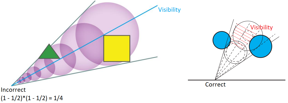
Evidently, by [McLaren 2015], the cone tracing may NOT dectect the full occlusion which is the result of mutiple partial occlusions.

References

[Jensen 2001] Henrik Jensen. "Realistic Image Synthesis Using Photon Mapping." AK Peters 2001.
[Hachisuka 2005] Toshiya Hachisuka. "High-Quality Global Illumination Rendering Using Rasterization." GPU Gems 2.
[Crassin 2011] Cyril Crassin, Fabrice Neyret, Miguel Sainz, Simon Green, Elmar Eisemann. "Interactive Indirect Illumination Using Voxel Cone Tracing." SIGGRAPH 2011.
[Dunn 2014] Alex Dunn. "Transparency (or Translucency) Rendering." NVIDIA GameWorks Blog 2014.
[Panteleev 2014] Alexey Panteleev. "Practical Real-Time Voxel-Based Global Illumination for Current GPUs." GTC 2014.
[McLaren 2015] James McLaren. "The Technology of The Tomorrow Children." GDC 2015.
[Takeshige 2015] Masaya Takeshige. "The Basics of GPU Voxelization." NVIDIA GameWorks Blog 2015.
[Eric 2017] Eric Arneback. “Comparing a Clipmap to a Sparse Voxel Octree for Global Illumination." Master thesis 2017.
[Heitz 2017] Eric Heitz. "Geometric Derivation of the Irradiance of Polygonal Lights." Technical report 2017.