Photon Mapping

Workflow

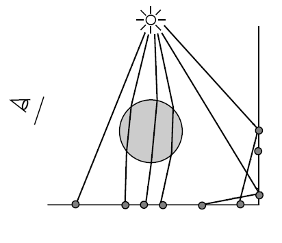
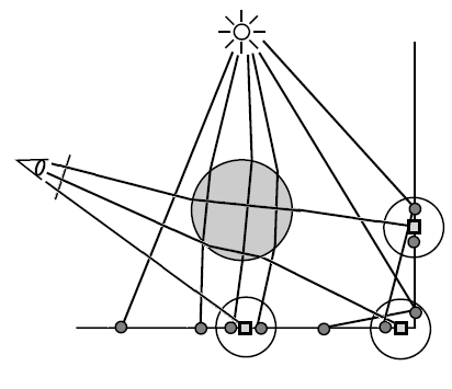
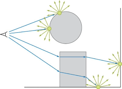
By "4.3 Overview" of [Jensen 2001] and "16.2.2 Photon Mapping" of PBR Book V3, the photon mapping is composed of two steps: photon tracing and rendering. During the photon tracing step, the photon rays are traced from the light sources, and the lighting information of the intersection positions of these photon rays is recorded as the photons. During the rendering step, the primary rays are traced from the camera and the final gather rays are traced from the final gather points, and the lighting information of the vicinal photons of the intersection positions of these primary rays or final gather rays is used to approximate the lighting of these intersection points by density estimation.

By "7.5 Photon Gathering" of [Jensen 2001], "38.2.2 Final Gathering" of [Hachisuka 2005] and "16.2.2 Photon Mapping" of PBR Book V3, the rendering step of the photon mapping is usually composed of two steps: radiance estimate and final gathering. During the radiance estimate step, the primary rays are traced from the camera, and the lighting information of the vicinal photons of the intersection positions of these primary rays is used to approximate the lighting of these intersection points by density estimation. During the final gathering step, from some of the intersection positions of the primary rays, which are called the final gather points, the final gather rays are traced, and the lighting information of the vicinal photons of the intersection positions of these final gather rays is used to approximate the lighting of these intersection positions by density estimation.

Photon Tracing	Rendering / Radiance-Estimate	Rendering / Final Gathering

Density Estimation

By "Equation (16.9)" of PBR Book V3, "Equation (7.3)" of [Jensen 2001] and "14.4.5 Delta Distributions in the Integrand" of PBR Book V3, we have $\displaystyle \operatorname{L_o}(\overrightarrow{p}, \overrightarrow{\omega_o}) = \int_{\mathrm{S}^2} \operatorname{f}(\overrightarrow{p}, \overrightarrow{\omega_i}, \overrightarrow{\omega_o}) \operatorname{L_i}(\overrightarrow{p}, \overrightarrow{\omega_i}) (\cos \theta_i)^+ \, d \overrightarrow{\omega_i} = \int_A \left\lparen \int_{\mathrm{S}^2} \operatorname{\delta}(\overrightarrow{p'} - \overrightarrow{p}) \operatorname{f}(\overrightarrow{p'}, \overrightarrow{\omega_i}, \overrightarrow{\omega_o}) \operatorname{L_i}(\overrightarrow{p'}, \overrightarrow{\omega_i}) (\cos \theta_i)^+ \, d \overrightarrow{\omega_i} \right\rparen \, d \operatorname{A}(\overrightarrow{p'})$ where $\displaystyle \operatorname{\delta}(\overrightarrow{p'} - \overrightarrow{p})$ is the delta function.

By "Equation (16.11)" of PBR Book V3 and "Equation (7.4)" of [Jensen 2001], the delta function is approximated by the filter function. This is the reason why the photon mapping algorithm is biased. Theoretically, the delta function is considered as an unknown probability density function, and the density estimation is used to approximate the probability density at the shading position. The kernel density estimation is one of the methods of the density estimation, and we have $\displaystyle \operatorname{L_o}(\overrightarrow{p}, \overrightarrow{\omega_o}) = \int_A \left\lparen \int_{\mathrm{S}^2} \operatorname{\delta}(\overrightarrow{p'} - \overrightarrow{p}) \operatorname{f}(\overrightarrow{p'}, \overrightarrow{\omega_i}, \overrightarrow{\omega_o}) \operatorname{L_i}(\overrightarrow{p'}, \overrightarrow{\omega_i}) (\cos \theta_i)^+ \, d \overrightarrow{\omega_i} \right\rparen \, d \operatorname{A}(\overrightarrow{p'}) \approx \sum_{i=1}^N \left\lparen \frac{1}{N} \frac{1}{h} \operatorname{K}(\frac{\overrightarrow{p_i} - \overrightarrow{p}}{h}) \right\rparen \left\lparen \int_{\mathrm{S}^2} \operatorname{f}(\overrightarrow{p}, \overrightarrow{\omega_i}, \overrightarrow{\omega_o}) \operatorname{L_i}(\overrightarrow{p_i}, \overrightarrow{\omega_i}) (\cos \theta_i)^+ \, d \overrightarrow{\omega_i} \right\rparen$ where $\displaystyle \frac{1}{h} \operatorname{K}(\frac{\overrightarrow{p_i} - \overrightarrow{p}}{h}) = \operatorname{K_h}(\overrightarrow{p_i} - \overrightarrow{p})$ is the scaled kernel. The k-NN (k-Nearest Neighbors) is one of the methods of the kernel density estimation, and is the actual method used by the photon mapping algorithm, and we have $\displaystyle \operatorname{L_o}(\overrightarrow{p}, \overrightarrow{\omega_o}) = \int_A \left\lparen \int_{\mathrm{S}^2} \operatorname{\delta}(\overrightarrow{p'} - \overrightarrow{p}) \operatorname{f}(\overrightarrow{p'}, \overrightarrow{\omega_i}, \overrightarrow{\omega_o}) \operatorname{L_i}(\overrightarrow{p'}, \overrightarrow{\omega_i}) (\cos \theta_i)^+ \, d \overrightarrow{\omega_i} \right\rparen \, d \operatorname{A}(\overrightarrow{p'}) \approx \frac{k}{N} \frac{1}{\pi {(\operatorname{R_k}(\overrightarrow{p}))}^2} \sum_{i=1}^N \int_{\mathrm{S}^2} \operatorname{f}(\overrightarrow{p}, \overrightarrow{\omega_i}, \overrightarrow{\omega_o}) \operatorname{L_i}(\overrightarrow{p_i}, \overrightarrow{\omega_i}) (\cos \theta_i)^+ \, d \overrightarrow{\omega_i}$ where $\displaystyle N = k \Rightarrow \frac{k}{N} = 1$ (the samples are exactly the k-nearest neighbors, namely, the number of the samples N is exactly the k), and $\displaystyle \operatorname{R_k}(\overrightarrow{p})$, which is also called the radius, is the maximum distance between each sample position $\displaystyle \overrightarrow{p_i}$ and the shading position $\displaystyle \overrightarrow{p}$ .

SPPM (Stochastic Progressive Photon Mapping)

"Equation (16.13)" of PBR Book V3

"SPPMIntegrator::Render" of PBRT V3

"24. Real-Time Global Illumination with Photon Mapping" of Ray Tracing Gems

"30. Caustics Using Screen Space Photon Mapping" of Ray Tracing Gems

"30. Real-Time Ray Traced Caustics" of Ray Tracing Gems II

References

[Jensen 2001] Henrik Jensen. "Realistic Image Synthesis Using Photon Mapping." AK Peters 2001.
[Hachisuka 2008] Toshiya Hachisuka, Shinji Ogaki, Henrik Jensen. "Progressive Photon Mapping." SIGGRAPH 2008.
[Hachisuka 2009] Toshiya Hachisuka, Henrik Jensen. "Stochastic Progressive Photon Mapping." SIGGRAPH 2009.