VXGI (Voxel Global Illumintaion)

1. Workflow

1-1. Photon Mapping

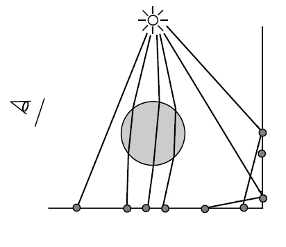
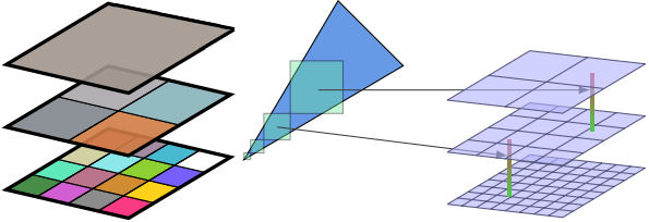
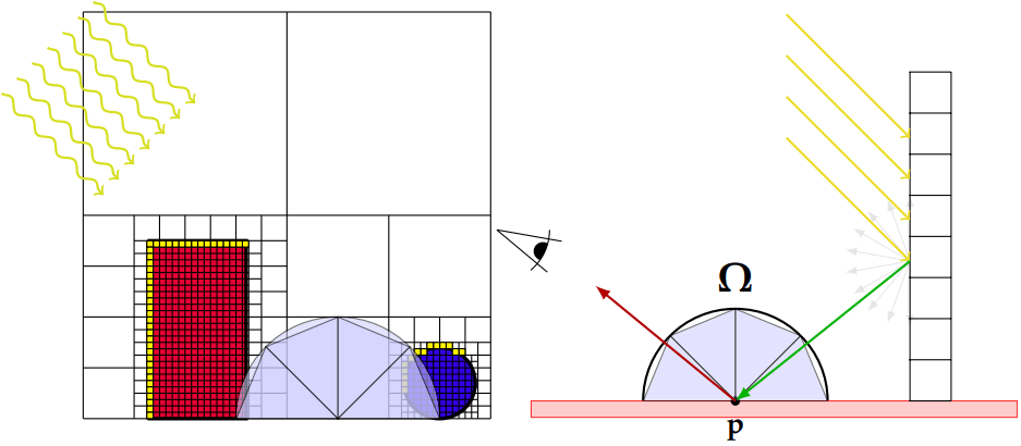
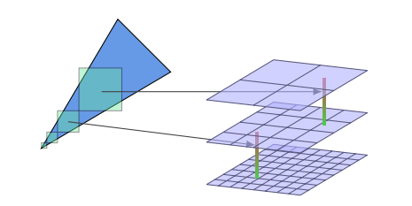
By "4.3 Overview" of [Jensen 2001] and "16.2.2 Photon Mapping" of PBR Book V3, the photon mapping is composed of two steps: photon tracing and rendering. During the photon tracing step, the photon rays are traced from the light sources, and the lighting information of the intersection positions of these photon rays is recorded as the photons. During the rendering step, the primary rays are traced from the camera and the final gather rays are traced from the final gather points, and the lighting information of the vicinal photons of the intersection positions of these primary rays or final gather rays is used to approximate the lighting of these intersection points by density estimation.

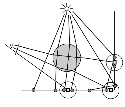
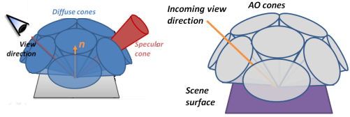
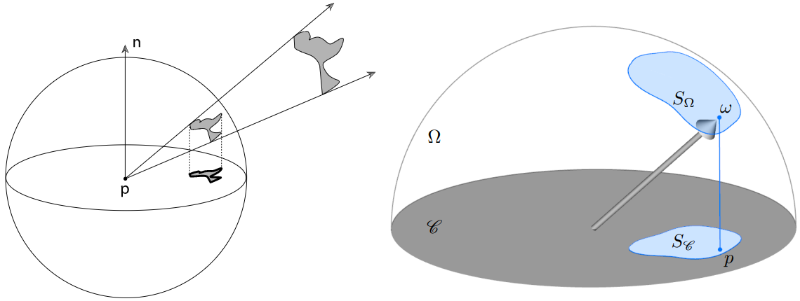
By "7.5 Photon Gathering" of [Jensen 2001], "38.2.2 Final Gathering" of [Hachisuka 2005] and "16.2.2 Photon Mapping" of PBR Book V3, the rendering step of the photon mapping is usually composed of two steps: radiance estimate and final gathering. During the radiance estimate step, the primary rays are traced from the camera, and the lighting information of the vicinal photons of the intersection positions of these primary rays is used to approximate the lighting of these intersection points by density estimation. During the final gathering step, from some of the intersection positions of the primary rays, which are called the final gather points, the final gather rays are traced, and the lighting information of the vicinal photons of the intersection positions of these final gather rays is used to approximate the lighting of these intersection positions by density estimation.

Photon Tracing	Rendering / Radiance-Estimate	Rendering / Final Gathering

1-2. VXGI (Voxel Global Illumintaion)

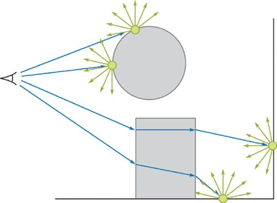
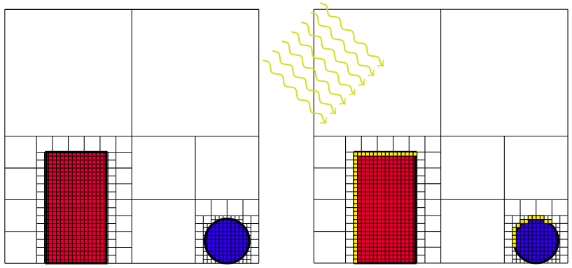
By [Crassin 2011 B], the VXGI (Voxel Global Illumintaion) is composed of three steps: light injection, filtering and cone tracing. The idea of the VXGI is intrinsically to implement the photon mapping by storing the photons in the voxels. The light injection step of the VXGI is analogous to the photon tracing step of the photon mapping. The cone tracing of the VXGI is analogous to the rendering / final gathering step of the photon mapping. The filtering step of the VXGI is analogous to the idea of the density estimation of the photon mapping.

Light Injection	Filtering	Cone Tracing

2-1. Light Injection

As per the original version by [Crassin 2011 B], the voxels are stored in the SVO (Sparse Voxel Octree). However, by [McLaren 2015] and [Eric 2017], the Clipmap is a better alternative. And actually, the Clipmap is exactly what the NVIDIA VXGI is based on.

2-1-1. Voxelization

By [Eric 2017], there are several approaches to inject the lighting. Some approaches treat the geometry and the lighting separablely. The geometry is voxelized at first, and then the RSM (Reflective Shadow Maps) by [Dachsbacher 2005] is used to inject the lighting later. The advantage of these approaches is that as long as the geometry remains the same, the voxelized data of the geometry can be reused even if the lighting has been changed. However, we will focus on the "voxelization-based" approach which the NVIDIA VXGI is based on. The light injection is performed at the same time when the geometry is voxelized. The most significant advantage of this approach is that the RSM is no longer required. However, the voxelized data can not be reused whenever either the geometry or the lighting has been changed. The VXGI::UpdateVoxelizationParameters::invalidatedRegions is used to invalidate the voxelized data when the geometry has been changed in the NVIDIA VXGI. And the VXGI::UpdateVoxelizationParameters::invalidatedLightFrusta is used to invalidate the voxelized data when the lighting has been changed in the NVIDIA VXGI.

2-1-2. Toroidal Addressing

TODO:
By [Panteleev 2014], the NVIDIA VXGI does use the Toroidal Addressing to reuse the voxelized data. However, it rarely happens that both the geometry and the lighting remain the same. Actually, the VXGI::VoxelizationParameters::persistentVoxelData is always set to false in the NVIDIA Unreal Engine 4 Fork. And the evolution of the rendering technique tends to get close to the real time solution and get rid of the cache based solution. The DXR (DirectX Raytracing) is the a typical example for this tendency. Thus, the Toroidal Addressing is not involved in the current version, but perhaps will be involved in the future version.

2-1-3. Clipmap Logical Structure

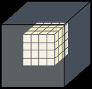
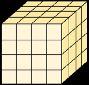
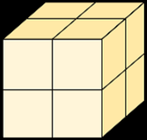
By [Panteleev 2014], we have the logical structure of the Clipmap. Each of the first several clipmap levels has only one mipmap level, and the last clipmap level is the only one which has multiple mipmap levels. The voxel size increases for each (clipmap or mipmap) level. The texture size (voxel count) (of the zeroth mipmap level) of each clipmap level is the same. The volume of each mipmap level of the same clipmap level is the same.

N/A	0-0	1-0	2-0	2-1	2-2
Figure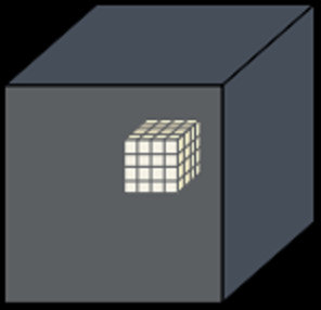
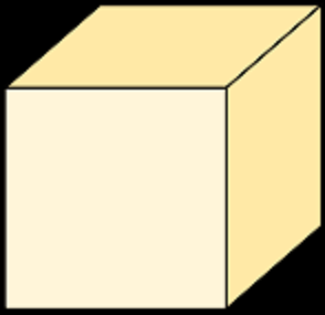Clipmap Level Index	0	1	2	2	2
Mipmap Level Index	0	0	0	1	2
Voxel Size	1	2	4	8	16
Texture Size (Voxel Count)	4	4	4	2	1
Volume	$\displaystyle (1 \times 4)^3 = 64$	$\displaystyle (2 \times 4)^3 = 512$	$\displaystyle (4 \times 4)^3 = 4096$	$\displaystyle (8 \times 2)^3 = 4096$	$\displaystyle (16 \times 1)^3 = 4096$

2-1-4. Clipmap Physical Structure

And here is the logical structure of the clipmap used in the Global Illumination sample of the NVIDIA VXGI. Each of the first four (index from 0 to 3) clipmap levels has only one mipmap level, and the last (index 4) clipmap level has six (index from 0 to 5) mipmap levels.

And here is the physical structure of the clipmap used in the Global Illumination sample of the NVIDIA VXGI. The clipmap is implemented by the $\displaystyle 128 \times 128 \times 785$ 3D texture.

2-1-4. MSAA

TODO: conservative rasterization
TODO: simulate "conservative rasterization" by MSAA ([Takeshige 2015])

TODO: not related to "ambient occlusion"

2-2. Filtering

TODO: anisotropic voxel

2-3. Cone Tracing

2-3-1. Monte Carlo Method

By Additive Interval Property, the ambient occlusion can be calculated as $\displaystyle \operatorname{k_A} = \int_\Omega \frac{1}{\pi} \operatorname{V}(\overrightarrow{\omega_i}) (\cos \theta_i)^+ \, d \overrightarrow{\omega_i} = \frac{1}{\pi} \sum_{i=0}^{n} \left\lparen \int_{\Omega_i} \operatorname{V}(\overrightarrow{\omega_i}) (\cos \theta_i)^+ \, d \overrightarrow{\omega_i} \right\rparen$ where n is the number of cones, and $\displaystyle \Omega_i$ is the solid angle subtended by the ith cone.

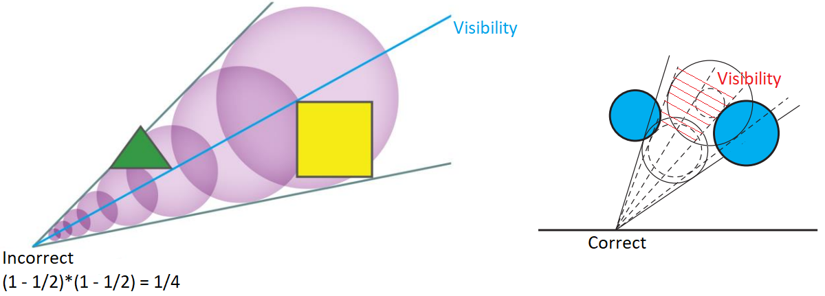
By [Crassin 2011 B], the visibility $\displaystyle \operatorname{V}(\overrightarrow{\omega_i})$ is assumed to be the same for all directions within the same cone, and the calculation of the ambient occlusion can be simplified as $\displaystyle \int_{\Omega_i} \operatorname{V}(\overrightarrow{\omega_i}) (\cos \theta_i)^+ \, d \overrightarrow{\omega_i} \approx \operatorname{V_c}(\Omega_i) \cdot \int_{\Omega_i} (\cos \theta_i)^+ \, d \overrightarrow{\omega_i}$ where $\displaystyle \operatorname{V_c}(\Omega_i) = 1 - \operatorname{A_{Final}}$ is the inverse of the final occlusion of the cone tracing.

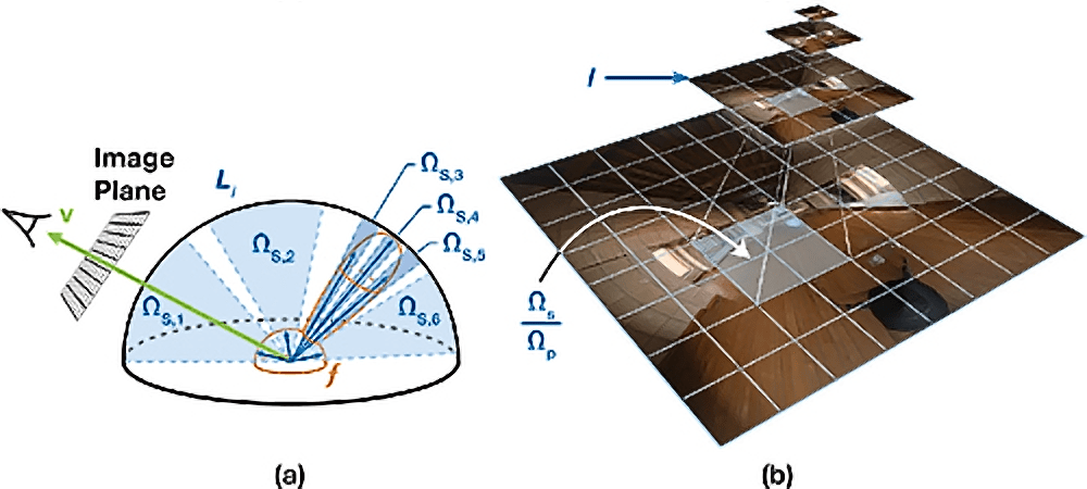
By "5.5.1 Integrals over Projected Solid Angle" of PBRT-V3 and [Heitz 2017], the integral of the clamped cosine $\displaystyle \int_{\Omega_i} (\cos \theta_i)^+ \, d \overrightarrow{\omega_i}$ can be calculated as the projected area on the unit disk.

By "20.4 Mipmap Filtered Samples" of [Colbert 2007], we use the mip-level $\text{sample\_mip\_level} = \displaystyle \max(0, \log(\sqrt{\frac{d\overrightarrow{\omega_S}}{d\overrightarrow{\omega_P}}}))$ to sample the filtered L value from the distant radiance distribution to reduce the variance. The $\displaystyle d\overrightarrow{\omega_S}$ is the solid angle subtended by the sample, and we have $\displaystyle d\overrightarrow{\omega_S} = \frac{1}{\text{N}} \cdot \frac{1}{\text{PDF}}$. The $\displaystyle d\overrightarrow{\omega_P}$ is the solid angle subtended by a single texel of the zeroth mip-level of the texture, and by "Projection from Cube Maps" of [Sloan 2008], we have $\displaystyle d\overrightarrow{\omega_P} = \frac{1}{\text{cubesize\_u} \cdot \text{cubesize\_v}} \cdot \frac{4}{\sqrt{1^2 + u^2 +v^2} \cdot (1^2 + u^2 +v^2)}$.

The $\displaystyle d\overrightarrow{\omega_S}$ is calculated by SolidAngleSample in UE4 and omegaS in Unity3D. And the $\displaystyle d\overrightarrow{\omega_P}$ is calculated by SolidAngleTexel in UE4 and invOmegaP in Unity3D.

2-3-2. Under Operator

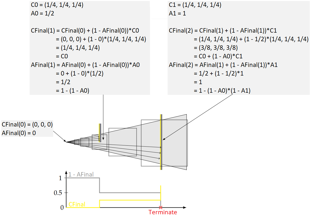
By [Crassin 2011 B], the under operator is used to calculated the final color $\displaystyle \mathrm{C}_\mathrm{Final}$ and the final occlusion $\displaystyle \mathrm{A}_\mathrm{Final}$ .

By [Dunn 2014], we have the recursive form of the under operator.
$\displaystyle \mathrm{C}_\mathrm{Final}^{0} = 0$
$\displaystyle \mathrm{A}_\mathrm{Final}^{0} = 0$
$\displaystyle \mathrm{C}_\mathrm{Final}^{n + 1} = \mathrm{C}_\mathrm{Final}^{n} + (1 - \mathrm{A}_\mathrm{Final}^{n}) \cdot \mathrm{C}_{n}$
$\displaystyle \mathrm{A}_\mathrm{Final}^{n + 1} = \mathrm{A}_\mathrm{Final}^{n} + (1 - \mathrm{A}_\mathrm{Final}^{n}) \cdot \mathrm{A}_{n}$

Actually, the explicit form of the under operator can be proved by mathematical induction.
$\displaystyle \mathrm{A}_\mathrm{Final}^{n + 1} = 1 - \prod_{i = 0}^{n} \left\lparen 1 - \mathrm{A}_{i} \right\rparen$
$\displaystyle \mathrm{C}_\mathrm{Final}^{n + 1} = \sum_{i = 0}^{n} \left\lparen \left\lparen \prod_{\mathrm{Z}_{j} \operatorname{Nearer} \mathrm{Z}_{i}} \left\lparen 1 - \mathrm{A}_{j} \right\rparen \right\rparen \cdot \mathrm{C}_{i} \right\rparen$

Evidently, by [McLaren 2015], the cone tracing may NOT dectect the full occlusion which is the result of mutiple partial occlusions.

2-3-3. Self Intersection

TODO

AdjustConePosition

By [Wachter 2019], "3.9.5 Robust Spawned Ray Origins" of PBR Book V3 and "6.8.6 Robust Spawned Ray Origins" of PBR Book V4, we should offset the ray origin to avoid self intersection.

References

[Jensen 2001] Henrik Jensen. "Realistic Image Synthesis Using Photon Mapping." AK Peters 2001.
[Hachisuka 2005] Toshiya Hachisuka. "High-Quality Global Illumination Rendering Using Rasterization." GPU Gems 2.
[Dachsbacher 2005] Carsten Dachsbacher, Marc Stamminger. "Reflective Shadow Maps." I3D 2005.
[Crassin 2011 A] Cyril Crassin. "GigaVoxels: A Voxel-Based Rendering Pipeline For Efficient Exploration Of Large And Detailed Scenes." PhD Thesis 2011.
[Crassin 2011 B] Cyril Crassin, Fabrice Neyret, Miguel Sainz, Simon Green, Elmar Eisemann. "Interactive Indirect Illumination Using Voxel Cone Tracing." SIGGRAPH 2011.
[Dunn 2014] Alex Dunn. "Transparency (or Translucency) Rendering." NVIDIA GameWorks Blog 2014.
[Panteleev 2014] Alexey Panteleev. "Practical Real-Time Voxel-Based Global Illumination for Current GPUs." GTC 2014.
[McLaren 2015] James McLaren. "The Technology of The Tomorrow Children." GDC 2015.
[Takeshige 2015] Masaya Takeshige. "The Basics of GPU Voxelization." NVIDIA GameWorks Blog 2015.
[Eric 2017] Eric Arneback. “Comparing a Clipmap to a Sparse Voxel Octree for Global Illumination." Master thesis 2017.
[Heitz 2017] Eric Heitz. "Geometric Derivation of the Irradiance of Polygonal Lights." Technical report 2017.